= incompleteBeta(a,b,x)
- (a−1)/(a+b−2) if a > 1 and b > 1
- 0 and 1 if a < 1 and b<1
- 0 if a < 1 and b ≥ 1
- 0 if a=1 and b > 1
- 1 if a ≥ 1 and b < 1
- 1 if a > 1 and b=1
- not defined if a=1 and b=1
http://www.physik.fu-berlin.de/~loison/finance/LOPOR/
Last update: March 2005
©Damien Loison, 2005
The LOPOR library is an efficient library for option pricing and operational risk. It is user-friendly and easy to use in combination with other libraries. For this reason, and contrary to all libraries that I know, no special type of variable is defined. Only types defined in the standard library std are used.
This manual is composed of two distinct parts.
The first part is devoted to present all tools necessary
to solve problems in option pricing and operational risk.
It is not a text book
and only a manual to use with the library.
With these tools you are able to solve any problem in operational
risk. For example see
[Vose2003,Marshall2001,Cruz2002].
The second part is devoted to option
pricing and could be considered as a text book with implementations.
It cannot be considered as exhaustive and is still in expansion.
If you are interested in this part,
I advice you strongly to read the section
Simple binomial model first.
It present some fundamental points of option pricing,
martingales and risk neutral considerations, through a very simple
example. It i very useful to understand these concepts in this case
before going to more complicated modelization.
This library could have some bugs. If you find one, please send me an email. Moreover if you do not find a function which could be useful for you, or if you do not understand something, please send me an email: Damien.Loison@physik.fu-berlin.de
All the library uses the LOPOR namespace. You have two ways to include the library:
"Our library is carefully made and extremely efficient …, obviously."
The errors are managed through the Error.hpp class. An Error is thrown if there is a problem. The syntax to throw one error is:
#include "Error.hpp"
#include "Global.hpp"
LOPOR::Error("define the error" + LOPOR::c2s(value) + "what you want" );
value can be a double, integer, boolean, etc. We use the function c2s( ) for "convert to string" defined in the class Global.hpp. To catch the Error the program must look like:
// Example Error1.cpp download
//
#include "LOPOR.hpp"
using namespace LOPOR;

int main( )
{
    try
    {
        Exponential exp;
        exp.setParameter(-2);
    }
    catch (const LOPOR::Error& error) { error.information( ); }
    return 0;
}
And the output of this program is:
Error: LOPOR::Exponential(-2)::setParameter( ) = > The variable:-2 must be > 0
We can replace error.information( ); by std::cout < < error.value << std::endl;
The class Random.hpp returns a random number between 0 and 1. There is no need create an instance of the class. You should use directly the static functions after having included the class with #include "Random.hpp"
| static double Random::ran( ) |
|
return a random number between 0 (included) and 1 (excluded) |
| static double Random::ranZero( ) |
|
return a random number between 0 (excluded) and 1 (excluded) |
| static vector <double> Random::ranVector(int n) |
|
return n random numbers between 0 (included) and 1 (excluded) |
| static void Random::setSeed(vector < int> seed) |
|
seed is a vector with 35 elements. The last two elements should not be zero. Usually used in combination with getSeed( ). |
| static vector < int> Random::getSeed( ) |
|
return a vector < int> with 35 elements. |
It is interesting to observe that some libraries propose to create many instances of the random generator with different seeds for each. This is wrong. The random numbers will not be independent and in particular if the choices of the seeds are in the same serie, there will be a very strong correlation between the different random numbers. If a library proposes this choice you could have some doubts about the reliability of the entire library.
To be able to run two programs successively with non correlated random numbers you should save the seed at the end of the first program using std::vector < int> s_fin=getSeed( ) and then set the seed at the beginning of the second program using setSeed(s_fin).
Following the last two paragraphs we can understand why to propose a function ranSeed( ) where the seed is initialized with the time or something else has no meaning. The computer is not luckier than you. To program a game it could be all right, but not in finance.
In this chapter we provide a way to obtain a random number generator for any distributions. This is in contrast with the majority of libraries which only give random number generators for predefined distributions. In addition to them, we give some classes to modify them (Homotecy, Multiply, Interval, Translate), to Sum them and also two general procedures, HeatBath and Hasting, to simulate any distributions.
The syntaxes of all distributions are alike. They are defined as a child
of the Distribution class defined in the file
"Distribution.hpp".
To use a class you can include the definitions of all
classes by #include "LOPOR.hpp"
or include the header file of the class like:
#include "Exponential.hpp" if we take the
Exponential distribution as example.
First you have to define an instance of the class:
Exponential exp
Then the functions that you can apply to this instance are:
| void setParameters(vector <double> parameters) |
|
define the parameters, for example : E=1/a exp(−x/a) with a=parameters[0]. The type and the number on parameters depends of the distribution. This function is defined in Distribution.hpp and inherited. Be careful of the name difference: this function is with "s" at the end, contrary to the next function. |
| void setParameter(double a, double b) |
|
define the parameters, for example : E=1/a exp(−x/a). The type and the number of parameters depends on the distribution. This function is not defined in Distribution.hpp and not inherited. The previous function is inherited. Be careful of the name difference: this one is without "s", the next with "s" at the end. |
| vector <double> get_Parameters( ) |
|
return a vector with all parameters of the distribution. |
| double ran( ) |
|
return a random number following the distribution. |
| vector <double> ranVector(int n) |
|
return n random numbers following the distribution. |
| vector <double> ranVectorLH(int n) |
|
return n random numbers following the distribution using the Latin Hypercube sampling. Give a better result than ranVector(n) but you must be cautious when using it: all the random numbers must be used to calculate the integrals. |
| double density(double x) |
|
return the density, called also the probability density or mass function. |
| vector <double> densityVector(vector<double > vec_x) |
|
return a vector with the density for each element of vec_x. |
| double cumulative(double x) |
|
return the cumulative distribution function F(x). F(x) varies from between 0 to 1. |
| vector <double> cumulativeVector(vector<double > vec_x) |
|
return a vector with the cumulative for each element of vec_x. |
| double mean( ) |
|
return the average. |
| double mode( ) |
|
return the mode. |
| double variance( ) |
|
return the variance. |
| double sigma( ) |
|
return the standard deviation = sqrt(variance( )) |
| double ran_fc(double y) |
|
return the inverse of the cumulative function
F−1(y) when it is known, with y between 0 and 1.
This function can be used to construct the function
ran( ): |
| std::string information( ) |
|
return information about the distribution. |
| vector <double> fit_keep |
|
This vector is used for the fit using the non linear functions LeastSquares_LM_cum( ) and LeastSquares_LM_den. Keep some parameters constant during the Fit. For example fit_keep={1,4} will keep the parameter number 1 (the second, the count begins at 0) and the number 4 (the fifth) constant. See Fit_LeastSquares_LM_cum2.cpp for an example. |
| vector <double> get_fit_keep_dist( ) |
|
return a vector with the constant parameters for the fit. For usual distribution return fit_keep. However if the distribution is constructed calling another distribution(s) like the class Translate, it is the sum of fit_keep of the distribution itself and the one from the called distribution. See an example in Fit_LeastSquares_LM_cum2.cpp |
| vector <double> get_fit_keep_cum_LM( ) |
|
return a vector with the constant parameters for the fit when using Fit_LeastSquares_LM_cum. It is implemented for each distribution. For example the vector {0,2} means that the first and third parameters will be kept constant during the fit. |
| vector <double> get_fit_keep_den_LM( ) |
|
return a vector with the constant parameters for the fit when using Fit_LeastSquares_LM_den. It is implemented for each distribution. For example the vector {0,2} means that the first and third parameters will be kept constant during the fit. |
An error is thrown if the function called does not exist.
Example of program:
// LOPOR.hpp include all the headers of the LOPOR library
#include "LOPOR.hpp"
using namespace LOPOR;

int main( )
{
    try
    {
                               // create an instance
        Exponential dist ;

                               // define the parameter a=2.
        dist.setParameter(2.);
                               // another possibility: create a vector
        dist.setParameters(c2v(2.));

                               // create the vector {0,1,2,3,…,9}
        std::vector <double>  vecX(vec_create(10,0.,1.));
                               // {f(0),f(1),…,f(9)}: f(x)=0.5 exp(-x/2)
        std::vector <double>  vecY(dist.densityVector(vecX));

                               // create a vector with 1000 random numbers
        std::vector <double> ranE(dist.ranVector(1000));

    }
    catch (const LOPOR::Error& error) { error.information( ); }
    return 0;
}
The information given in this chapter comes mainly from [Johnson1994a] and [Evans2000].
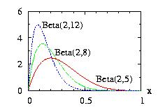
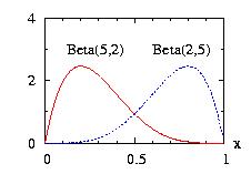
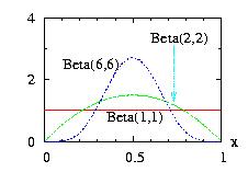
| class: | Beta.hpp |
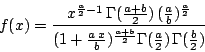
| density: |
|
| restrictions: | a > 0, b > 0 |
| domain: | 0 ≤ x ≤ 1 |
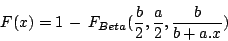
| cumulative: |
= incompleteBeta(a,b,x) |
| mean: | a/(a+b) |
| mode: |
|
| variance: | a.b.(a+b)−2.(a+b+1)−1 |
In addition to the general syntax, we have:
| void setParameter(double a, double b) | a > 0, b > 0 |
|
vector <double> E.ranVectorLH(int n); double E.ran_fc(double y); |
not defined an Error is thrown when called. |
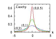
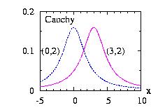
| class: | Cauchy.hpp |
| density: | f(x) = ( b2+(x−a)2 )−1/(π b) |
| restrictions: | b > 0 |
| domain: | −∞ < x < +∞ |
| cumulative: | F(x) = 0.5 + π−1 tan−1 ( (x−a) b−1 ) |
| mean: | not defined |
| mode: | a |
| variance: | not defined |
In addition to the general syntax, we have:
| void setParameter(double a, double b) | b positive. |
|
double mean( ) double variance( ) double sigma( ) |
not defined an Error is thrown when called. |
| vector <double> Moments(Distribution* dist,vector <double> vecX) |
not defined an Error is thrown when called. |
All the other fit functions described in Fit are accessible.
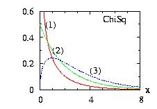
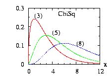
| class: | ChiSq.hpp |
| density: |
  |
| restrictions: | a > 0 |
| domain: | x > 0; |
| cumulative: | incompleteGamma(a/2,x/2) |
| mean: | a |
| mode: |
|
| variance: | 2 a |
In addition to the general syntax, we have:
| void setParameter(double a, double b) | a > 0 |
|
vector <double> E.ranVectorLH(int n); double E.ran_fc(double y); |
not defined an Error is thrown when called. |
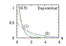
| class: | Exponential.hpp |
| density: | f(x) = a-1 exp(− x/a) |
| restrictions: |
a > 0 |
| domain: | x > 0 |
| cumulative: | F(x) = 1 − exp(−x/a) |
| mean: | a |
| mode: | 0 |
| variance: | a2 |
In addition to the general syntax, we have:
| void setParameter(double a) |
a > 0 |
| class: |
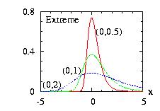
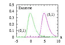
Extreme.hpp Known also as Gumbel distribution |
| density: | f(x) = b−1 exp[ −(x−a)/b − exp(−(x−a)/b) ] |
| restrictions: | b > 0 |
| domain: | −∞ < x < +∞ |
| cumulative: | F(x) = exp[ − exp(−(x−a)/b) ] |
| mean: | a − b Γ'(1) |
| mode: | a |
| variance: | b2 π2/6 |
In addition to the general syntax, we have:
| void setParameter(double a, double b) | b > 0. |
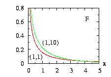
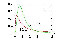
| class: | F.hpp |
| density: |
 |
| restrictions: |
a > 0 b > 0 |
| domain: | 0 < x < +∞ |
| cumulative: |
  |
| mean: | b/(b − 2) if b > 2 |
| mode: | b/a . (a − 2)/(b + 2) if a > 2 |
| variance: | 2 b2 (a + b − 2)/ [ a (b − 2)2 (b − 4) ] if b > 4 |
In addition to the general syntax, we have:
| void setParameter(double a, double b) |
a > 0. b > 0. |
|
vector <double> E.ranVectorLH(int n); double E.ran_fc(double y); |
not defined an Error is thrown when called. |
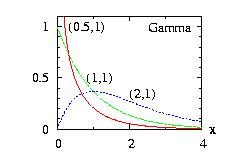
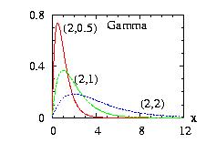
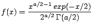
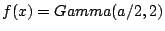
| class: | Gamma.hpp |
| density: | xa−1 exp(−x/b) /( Γ(a) ba ) |
| restrictions: | a > 0 and b > 0 |
| domain: | 0 ≤ x |
| cumulative: | incompleteGamma(a,x/b) |
| mean: | a b |
| mode: |
|
| variance: | a b2 |
In addition to the general syntax, we have:
| void setParameter(double a, double b) | a and b positive. |
|
vector <double> E.ranVectorLH(int n); double E.ran_fc(double y); |
not defined an Error is thrown when called. |
The x coordinates are not necessary equidistant. However in
this case the calls to the functions density(x) and cumulative(x) are slower.
We use the Walker class to calculate
the properties of this class.
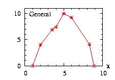
| class: | General.hpp |
| density: |
f(x) = pi +
(pi+1−pi)
(x−xi) / (xi+1−xi) i is an integer from 0 to n−1 |
| restrictions: |
n ≥ 1 pi ≥ 0 and at least one pi ≠ 0; p has n components xi < xi+1; x has n components |
| domain: | x0 ≤ x ≤ xn−1 |
| cumulative: | |
| mean: | |
| mode: | no closed form |
| variance: |
In addition to the general syntax, we have:
|
void setParameter ( vector <double> x, vector <double> p) |
x and p have n components. See restrictions above. |
| int get_i ( double x ) | return the number of the interval (0 to n−1) corresponding to the value x. |
|
vector <double> E.ranVectorLH(int n); double E.ran_fc(double y); |
not defined an Error is thrown when called. |
Fit No fit functions described in Fit are accessible.
The x coordinates are not necessary equidistant. However in
this case the calls to the functions density(x) and cumulative(x) are slower.
We use the Walker class to calculate
the properties of this class.
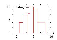
| class: | Histogram.hpp |
| density: | f(x) = pi if xi ≤ x < xi+1 i is an integer from 0 to n−1 |
| restrictions: |
n ≥ 2 pi ≥ 0 and at least one pi ≠ 0, there are n−1 probabilities pi xi < xi+1, there are n values xi |
| domain: | x0 ≤ x ≤ xn−1 |
| cumulative: | |
| mean: | |
| mode: | no closed form |
| variance: |
In addition to the general syntax, we have:
|
void setParameter ( vector <double> x, vector <double> p) |
x and p have n components and n−1 components, respectively. See restrictions above. |
| int get_i ( double x ) | return the number of the interval (0 to n−1) corresponding to the value x. |
|
vector <double> E.ranVectorLH(int n); double E.ran_fc(double y); |
not defined an Error is thrown when called. |
Fit
No fit functions described in Fit are accessible.
A related class is the StepFunction class.
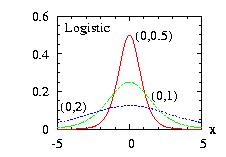
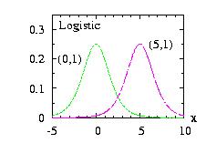
| class: | Logistic.hpp |
| density: |
f(x) = z b−1 (1 + z)−2 with z = exp[ − (x − a) / b ] |
| restrictions: | b > 0 |
| domain: | −∞ < x < +∞ |
| cumulative: | F(x) = ( 1 + z )−1 |
| mean: | a |
| mode: | a |
| variance: | b2 π2 / 3 |
In addition to the general syntax, we have:
| void setParameter(double a, double b) | b > 0. |
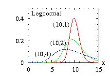
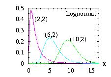
| class: | Lognormal.hpp |
| density: |
f(x) = x−1
( 2 π σ2 )−1/2
exp[
− ( log( x ) − μ )2 / ( 2
σ2 )
] μ = log [ a2 / ( b2 + a2 )1/2 ] σ = [ log( (b2 + a2 ) / a2 ) ]1/2 |
| restrictions: | a > 0 and b > 0 |
| domain: | 0 ≤ x |
| cumulative: | Normalcumulative( (log(x)-μ)/σ ) |
| mean: | a |
| mode: | exp( μ − σ2 ) |
| variance: | b2 |
In addition to the general syntax, we have:
| void setParameter(double a, double b) | a > 0 and b > 0 |
|
vector <double>
E.ranVectorLH(int n); double E.ran_fc(double y); double E.cumulative(double x); |
not defined an Error is thrown when called. |
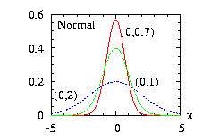
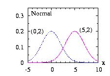
| class: | Normal.hpp |
| density: | f(x) = ( 2 π σ2 )−1/2 exp[ − (x − μ)2 / ( 2 σ2 ) ] |
| restrictions: | σ > 0 |
| domain: | −∞ < x < +∞ |
| cumulative : | 0.5+0.5*incompleteGamma( 0.5 , (x − μ)2 / (2 σ2) ) * sign(x − μ) |
| mean: | μ |
| mode: | μ |
| variance: | σ2 |
In addition to the general syntax, we have:
| void setParameter(double μ, double σ) |
|
μ > 0 |
|
static double
static_ran(double mean=0, double var=1); |
|
Static function. Return a random number from a normal distribution with the mean and the variance given as parameter. |
| static vector <double> static_ranVector(int n); |
|
Static function. Return n random numbers following the Normal distribution. |
|
static double
static_density(double x, double mean=0, double var=1); |
|
Static function. Return the density of a normal distribution with the mean and the variance given as parameter. |
|
static double
static_cumulative(double x, double mean=0, double var=1); |
|
Static function. Return the cumulative of a normal distribution with the mean and the variance given as parameter. |
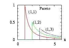
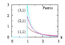
| class: | Pareto.hpp |
| density: | f(x) = θ aθ x−θ−1 |
| restrictions: | θ > 0 and a > 0 |
| domain: | a ≤ x |
| cumulative: | F(x) = 1 − (a/x)θ |
| mean: | a θ / (θ − 1) |
| mode: | a |
| variance: | a2 θ (θ −1)−2 (θ −2)−1 |
In addition to the general syntax, we have:
| void setParameter(double θ, double a) | θ > 0 and a > 0 |
| vector <double> Moments(Distribution* dist,vector <double> vecX) |
not defined an Error is thrown when called. |
All the other fit functions described in Fit are accessible.
The Rayleigh is the Weibull distribution with a = 2.
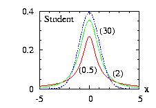
| class: | Student.hpp |
| density: |
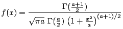 |
| restrictions: | a > 0 |
| domain: | −∞ < x < +∞ |
| cumulative: |
0.5+0.5*( incompleteBeta(a/2,0.5,1)−
incompleteBeta(a/2,0.5,a/(a+x*x)) )*sign(x) |
| mean: | 0 if a > 1 |
| mode: | 0 |
| variance: | a / (a − 2) |
In addition to the general syntax, we have:
| void setParameter(double a) | a positive. |
|
vector <double> E.ranVectorLH(int n); double E.ran_fc(double y); double E.cumulative(double x); |
not defined an Error is thrown when called. |
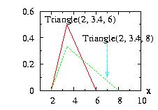
It is similar to the General
class with 2 sections.
| class: | Triangle.hpp |
| density: |
f(x) = 2 (x − a)
(b − a)−1
(c − a)−1
if a ≤ x ≤ b f(x) = 2 (c − x) (c − a)−1 (c − b)−1 if b < x ≤ c |
| restrictions: | a ≤ b ≤ c and a < c |
| domain: | a ≤ x ≤ c |
| cumulative: |
F(x) = 0 if x < a F(x) = (x − a)2 (b − a)−1 (c − a)−1 if a ≤ x ≤ b F(x) = 1 − (c − x)2 (c − a)−1 (c − b)−1 if b < x ≤ c F(x) = 1 if c < x |
| mean: | (a + b + c)/3 |
| mode: | b |
| variance: | (a2 + b2 + c2 − a b − a c − b c)/18 |
In addition to the general syntax, we have:
| void setParameter(double a, double b, double c) | a ≤ b ≤ c and a < c |
Fit No fit functions described in Fit are accessible.
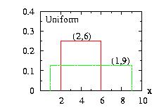
| class: | Uniform.hpp |
| density: | f(x)= 1/(b − a) if a ≤ x ≤ b |
| restrictions: | a < b |
| domain: | a ≤ x ≤ b |
| cumulative: |
F(x) = 0 if x < a F(x) = (x − a) / (b − a) if a ≤ x ≤ b F(x) = 1 if b < x |
| mean: | (a + b)/2 |
| mode: | not defined |
| variance: | (b − a)2 / 12 |
In addition to the general syntax, we have:
| void setParameter(double a, double b) | a ≤ b |
|
double mode( ); |
not defined an Error is thrown when called. |
Fit No fit functions described in Fit are accessible.
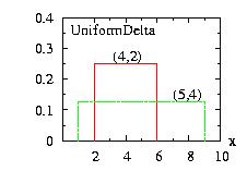
| class: | UniformDelta.hpp |
| density: | f(x)= 1/(2 δ ) if xi − δ ≤ x ≤ xi + δ |
| restrictions: | |
| domain: | xi − δ ≤ x ≤ xi + δ |
| cumulative: |
F(x) = 0 if x < xi − δ F(x) = (x − xi + δ) / (2 δ) if xi − δ ≤ x ≤ xi + δ F(x) = 1 if x > xi + δ |
| mean: | xi |
| mode: | not defined |
| variance: | δ2 / 3 |
In addition to the general syntax, we have:
| void setParameter(double xi, double δ) | |
| void setParameter(double xi) | The parameter δ keeps its value. If δ not already defined, δ=1 automatically. |
| void ran_(double xi) | identical to ran() but the xi is updated before the call of ran() |
|
double mode( ); |
not defined an Error is thrown when called. |
This class should not be used with the Interval class.
Never program something like that:
//WRONG
UniformDelta uniDel;
uniDel.setParameter(0,1);

Interval interval;
interval.setParameter(&uniDel,0,10,2);
It will not work, the xi in uniDel will not be updated.
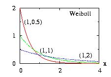
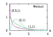
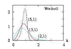
| class: | Weibull.hpp |
| density: | f(x)= a b−a xa−1 exp( −(x/b)a ) |
| restrictions: | a > 0 and b > 0 |
| domain: | x > 0 |
| cumulative: | F(x)= 1 − exp( −(x/b)a ) |
| mean: | Γ(1/a) b/a |
| mode: | b (1 − 1/a)1/a |
| variance: | [ 2 Γ(2/a) − Γ(1/a)2 /a ] b2/a |
In addition to the general syntax, we have:
| void setParameter(double a, double b) | a > 0 and b > 0 |
Information given in this chapter comes mainly from [Johnson1994b] and [Evans2000].
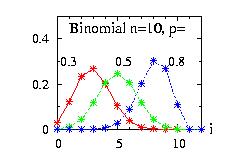
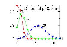
| class: | Binomial.hpp |
| density: |
|
| restrictions: | 0 < p < 1 and n={0,1,2,…} |
| domain: | x ∈ {0,1,2,…,n} |
| cumulative: |
|
| mean: | n p |
| mode: |
|
| variance: | n p (1 − p) |
In addition to the general syntax, we have:
| void setParameter(int n, double p) | 0 < p < 1 and n={0,1,2,…} |
|
vector <double> E.ranVectorLH(int n); double E.ran_fc(double y); |
not defined an Error is thrown when called. |
Fit
All fit functions described in Fit are accessible.
Moreover the fit_keep is initialized with the constraint
that the
first parameter of the class, n, is kept const when using
LeastSquares_LM_cum
and LeastSquares_LM_den.
The ran( ) function is on the form double. You
should use the function LOPOR::
c2floor( ) provided in the
class Global to get the integer.
Similarly with the ranVector( )
function
you should use the function vec_c2floor( ) provided in the class
Vector.
Example of program:
// Example Binomial1.cpp download
//
#include "LOPOR.hpp"
using namespace LOPOR;

int main( )
{
    try
    {
        Binomial bino;
        bino.setParameter(10,0.2);

        // print 1 random number
        print("bino.ran( )=",c2floor(bino.ran( )));

        // print 10 random numbers
        vec_print(vec_c2floor(bino.ranVector(10)),"results ");
    }
    catch (const LOPOR::Error& error) { error.information( ); }
    return 0;
}
The output of this program is:
bino.ran( )= 1
#   i=      results
     0              3
     1              3
     2              2
     3              3
     4              1
     5              2
     6              4
     7              1
     8              1
     9              4
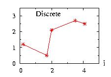
| class: | Discrete.hpp |
| density: |
f(xi) = pi integer i from 0 to n−1 |
| restrictions: |
n ≥ 1 pi ≥ 0 and at least one pi ≠ 0, there are n probabilities pi xi < xi+1, there are n values xi |
| domain: | x ∈ {x0,x1,…,xn} |
| cumulative: | F(xi) = p0 + p1 + … + pi |
| mean: | ( p0 x0 + p1 x1 + … pn−1 xn−1 ) / n |
| mode: | |
| variance: | ( p0 (x0 − mean)2 + p1 (x1 − mean)2 + … + pn−1 (xn−1 − mean)2 )/ n |
In addition to the general syntax, we have:
| void setParameter(vector <int> x, vector <double> double p) | x and p have n elements. |
| void setParameter(vector <int> x) | x has n elements. All the {pi} are equal: pi=1/n; |
|
double ran_fc(double y); |
not defined an Error is thrown when called. |
Fit
No fit functions described in Fit are accessible.
The class uses the Walker
procedure.
The ran( ) function is on the form double. You
should use the function LOPOR::c2floor( ) to get the integer.
Similarly with the ranVector( )
function
you should use the function vec_c2floor( ) provided in the class
Vector.
Example of program:
// Example Discrete1.cpp download
//
#include "LOPOR.hpp"
using namespace LOPOR;

int main( )
{
    try
    {
        Discrete disc;
        disc.setParameter(c2v<double>(0.2,1.7,2.0,3.5,4.1),
                                   c2v<double>(1.2,0.5,2.1,2.7,2.5));

        // print 1 random number
        print("disc.ran( )=",disc.ran( ));

        // print 10 random numbers
        vec_print(disc.ranVector(10),"results ");
    }
    catch (const LOPOR::Error& error) { error.information( ); }
    return 0;
}
The output of the program is:
disc.ran( )= 4.1
#   i=      results
     0            0.2
     1            1.7
     2            4.1
     3              2
     4              2
     5            4.1
     6            3.5
     7            3.5
     8              2
     9            0.2
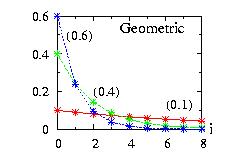
| class: | Geometric.hpp |
| density: |
f(i) = p (1 − p)i |
| restrictions: | 0 < p ≤ 1 |
| domain: | integer i ≥ 0 |
| cumulative: | F(i) = 1 − (1 − p)i+1 |
| mean: | (1 − p) / p |
| mode: | 0 |
| variance: | (1 − p) / p2 |
In addition to the general syntax, we have:
| void setParameter(double p) | 0 < p ≤ 1 |
Fit
All fit functions described in Fit are accessible.
Moreover the fit_keep is initialized
with the constraint that the
first parameter of the class, n, is kept const when using
LeastSquares_LM_cum
and LeastSquares_LM_den.
The ran( ) function is on the form double. You
should use the function LOPOR::c2floor( ) to get the integer.
Similarly with the ranVector( )
function
you should use the function vec_c2floor( ) provided in the class
Vector.
Example of program:
// Example Geometric1.cpp download
//
#include "LOPOR.hpp"
using namespace LOPOR;

int main( )
{
    try
    {
        Geometric geo;
        geo.setParameter(0.3);

        // print 1 random number
        print("geo.ran( )=",c2floor(geo.ran( )));

        // print 10 random numbers
        vec_print(vec_c2floor(geo.ranVector(10)),"results ");
    }
    catch (const LOPOR::Error& error) { error.information( ); }
    return 0;
}
The output of this program is:
geo.ran( )= 6
#   i=      results
     0              0
     1              0
     2              0
     3              1
     4              2
     5              1
     6              3
     7              3
     8              1
     9              0
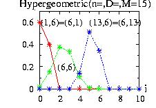
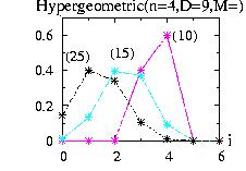
| class: | Hypergeometric.hpp |
| density: |
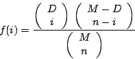
|
| restrictions: |
0 < n ≤ M 0 < D ≤ M M > 0 D, M, n integer |
| domain: |
integer i ≥ 0 maximum(0,n + D − M) ≤ i ≤ minimum(n,D) |
| cumulative: |
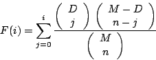
|
| mean: | n D / M |
| mode: | no closed form |
| variance: | D (M − D) n /M2 |
In addition to the general syntax, we have:
| void setParameter(int n, int D, int M) | see restriction above |
| double mode( ) | test all i, can be time consuming |
|
vector <double> E.ranVectorLH(int n); double E.ran_fc(double y); |
not defined an Error is thrown when called. |
Fit
No fit functions described in Fit are accessible.
The ran( ) function is on the form double. You
should use the function LOPOR::c2floor( ) to get the integer.
Similarly with the ranVector( )
function
you should use the function vec_c2floor( ) provided in the class
Vector.
Example of program: see Geometric1.cpp.
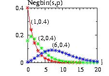
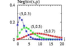
| class: | Negbin.hpp |
| density: |
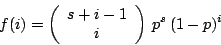
|
| restrictions: |
integer s > 0 0 < p ≤ 1 |
| domain: |
integer i ≥ 0 |
| cumulative: |
|
| mean: | s (1 − p) / p |
| mode: |
z and z+1 if z is an integer (int)(z+1) otherwise z=( s (1 − p) − 1 ) / p |
| variance: | s (1 − p) / p2 |
Note: for s=1 the negative binomial distribution is equivalent to the
geometric distribution:
Negbin (1,p)=Geometric(p)
In addition to the general syntax, we have:
| void setParameter(int s, double p) | see restriction above |
|
vector <double> E.ranVectorLH(int n); double E.ran_fc(double y); |
not defined an Error is thrown when called. |
Fit
All fit functions described in Fit are accessible.
Moreover the fit_keep is initialized that the
first parameter of the class, s, is kept const when using
LeastSquares_LM_cum
and LeastSquares_LM_den.
The ran( ) function is on the form double. You
should use the function LOPOR::c2floor( ) to get the integer.
Similarly with the ranVector( )
function
you should use the function vec_c2floor( ) provided in the class
Vector.
Example of program: see Geometric1.cpp.
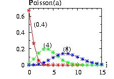
| class: | Poisson.hpp |
| density: |

|
| restrictions: | a > 0 |
| domain: |
integer i ≥ 0 |
| cumulative: |
|
| mean: | a |
| mode: |
a, a − 1 if a is an integer (int)(a) otherwise |
| variance: | a |
In addition to the general syntax, we have:
| void setParameter(double a) | a > 0 |
|
vector <double> E.ranVectorLH(int n); double E.ran_fc(double y); |
not defined an Error is thrown when called. |
The ran( ) function is on the form double. You
should use the function LOPOR::c2floor( ) to get the integer.
Similarly with the ranVector( )
function
you should use the function vec_c2floor( ) provided in the class
Vector.
Example of program: see Geometric1.cpp.
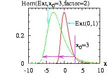 The class Homotecy.hpp allows you to make a homotocy
around a point x0 by a factor that you
give:
The class Homotecy.hpp allows you to make a homotocy
around a point x0 by a factor that you
give:
(x − x0) → (x − x0).factor
then the new instance Homotecy(&distribution,x0,factor)
can be used as an usual distribution.
In addition to the general
syntax, we have:
| void setParameter(Distribution* d, double x0, double factor); |
|
where Distribution* is the address of the distribution to transform. |
| void refresh( ); |
|
if the distribution (Extreme in our example) has changed you should refresh the class. This is not done automatically because it is very time consuming to check it at each call of ran( ) Moreover the call of refresh( ) call the refresh( ) function of the distribution given as parameter. |
Fit
All fit functions described in Fit are accessible.
Moreover the fit_keep is initialized with the constraint
that the
first parameter of the class, x0, is kept const when using
LeastSquares_LM_cum
and LeastSquares_LM_den.
The program to
generate the figure above could be:
// Example Homotecy1.cpp download
//
#include "LOPOR.hpp"
using namespace LOPOR;

int main( )
{
    try
    {
        Extreme Ext;
        Ext.setParameter(0,1);
        Homotecy Hom;
        Hom.setParameter(&Ext,3,2);

        // vecX={-10, -9.99, -9.98,…, 9.99, 10}
        std::vector<double> vecX(vec_create(2001,-10.,0.01));

        // to create the figure above:
        // print in file "Homotecy1.res", the vectors:
        // i           vecX   density(Extreme) density(Homotecy)
        // 0            -10              0      1.37459e-13
        // 1          -9.99              0      1.61336e-13
        // 2          -9.98             …     ….
        vec_print("Homotecy1.res",vecX,Ext.densityVector(vecX),
                          Hom.densityVector(vecX));

        // print 10 random numbers
        vec_print(Hom.ranVector(10),"results ");
    }
    catch (const LOPOR::Error& error) { error.information( ); }
    return 0;
}
And the program will create the file "Homotecy1.res" used to plot the figure above and print on the screen:
#   i=      results
     0        1.52601
     1       -5.81126
     2       -3.90537
     3       -3.49595
     4       -2.61605
     5        -1.9611
     6       -3.30339
     7       -1.24151
     8       -0.72952
     9       -2.50452
The class Interval.hpp allows you to choose an interval [A,B] where the function is zero outside of it. There are three possible values of the border for Interval(&distribution,A,B,border). We take as example in the figure A=−1, B=+2.
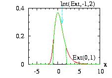
border=0: (by default)
f(x) → f(x) if A ≤ x ≤ B
f(x) → 0 if x < A or B < x
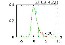
border=1:
f(x) → f(x) if −∞ < x ≤ B
f(x) → 0 if B < x
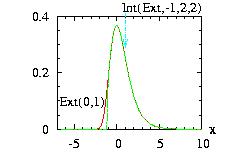
border=2:
f(x) → f(x) if A ≤ x < −∞
f(x) → 0 if x < A
then the new instance Interval(&distribution,A,B,border)
can be used at an usual distribution.
In addition to the general
syntax, we have:
| void setParameter(Distribution* d, double A, double B, double border=0); |
|
where Distribution* is the address of the distribution to transform. |
double successPerCent( );
|
|
return the percentage of success of the calls for ran( ) and ranVector( ) functions of the new interval instance. These functions can be produced in two ways:
|
| void refresh( ); |
|
if the distribution (Extreme in our example) has changed, you should refresh the class. This is not done automatically because it is very time-consuming to check it at each call of ran( ). Moreover the call of refresh() calls the refresh( ) function of the distribution given as parameter. |
| vector <double> Moments(Distribution* dist,vector <double> vecX) |
|
not defined |
| vector <double> MLE(Distribution* dist,vector <double> vecX) |
|
not defined |
All the other fit functions described in Fit are accessible.
The program to generate the second figure above could be:
// Example Interval1.cpp download
//
#include "LOPOR.hpp"
using namespace LOPOR;

int main( )
{
    try
    {
        Extreme Ext;
        Ext.setParameter(0,1);
        Interval Int;
        Int.setParameter(&Ext,-1,2,1);

        // vecX={-7, -6.99, -9.98,…, 9.99, 10}
        std::vector<double> vecX(vec_create(1701,-7.,0.01));

        // to create the figure above:
        // print in file "Interval1.res", the vectors:
        // i           vecX   density(Extreme) density(Interval)
        // 0            -7               0      0
        // 1          -6.99              0      0
        // 2          -6.98             …     ….
        vec_print("Interval1.res",vecX,Ext.densityVector(vecX),
                   Int.densityVector(vecX));

        // print 10 random numbers
        vec_print(Int.ranVector(10),"ran ");
    }
    catch (const LOPOR::Error& error) { error.information( ); }
    return 0;
}
And the program will create the file "Interval1.res" used to plot the figure above and print on the screen:
#   i=      ran
     0        1.42973
     1       -1.43828
     2      -0.535245
     3      -0.348377
     4      0.0401327
     5        0.31446
     6      -0.261702
     7       0.597054
     8       0.783772
     9      0.0878482
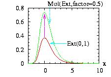 The class Multiply.hpp allows you to multiply the density
function by a positive factor.
The class Multiply.hpp allows you to multiply the density
function by a positive factor.
f(x) → f(x).factor
then the new instance, Multiply(&distribution,factor),
can be used at an usual distribution. This does not change
the way of producing the random number from this
distribution. However it will have an influence when we add
the distribution with the Sum class and
with the HeatBath class.
In addition to the general
syntax, we have:
| void setParameter(Distribution* d, double factor); |
|
where Distribution* is the address of the distribution to transform. |
| void refresh( ); |
|
if the distribution (Extreme in our example) has changed, you should refresh the class. This is not done automatically because it is very time-consuming to check it at each call of ran( ). Moreover the call of refresh() calls the refresh( ) function of the distribution given as parameter. |
Fit
All fit functions described in Fit are accessible.
Moreover the fit_keep vector is initialized with
the constraint that the
last parameter of the class, factor, is kept constant when using
LeastSquares_LM_cum.
The program to generate the figure above could be:
// Example Multiply1.cpp download
//
#include "LOPOR.hpp"
using namespace LOPOR;

int main( )
{
    try
    {
        Extreme Ext;
        Ext.setParameter(0,1);
        Multiply Mul;
        Mul.setParameter(&Ext,2);

        // vecX={-3, -2.99, -2.98,…, 9.99, 10}
        std::vector<double> vecX(vec_create(1301,-3.,0.01));

        // to create the figure above:
        // print in file "Multiply1.res", the vectors:
        // i           vecX   density(Extreme) density(Multiply)
        // 0             -3   3.80054e-08      7.60109e-08
        // 1          -2.99   4.59514e-08      9.19027e-08
        // 2          -2.98             …     ….
        vec_print("Multiply1.res",vecX,Ext.densityVector(vecX),
                      Mul.densityVector(vecX));

        // print 10 random numbers
        vec_print(Mul.ranVector(10),"ran ");
    }
    catch (const LOPOR::Error& error) { error.information( ); }
    return 0;
}
And the program will create the file "Multiply1.res" used to plot the figure above and print on the screen:
#   i=      ran
     0        2.26301
     1       -1.40563
     2      -0.452687
     3      -0.247977
     4       0.191976
     5       0.519449
     6      -0.151694
     7       0.879247
     8        1.13524
     9       0.247738
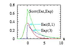 The class Sum.hpp allows you to add several distributions.
f1(x), f2(x) … → f1(x) + f2(x) + …
then the new instance, Sum(vector < &distribution > ),
can be used at an usual distribution.
In addition to the general
syntax, we have:
| void setParameter( vector <Distribution*> d); |
|
where d={d1,d2,…} is a vector composed of the addresses of the distributions to add. |
| void refresh( ); |
|
if the distribution (Extreme and Exponential in our example) has changed, you should refresh the class. This is not done automatically because it is very time-consuming to check it at each call of ran( ). Moreover the call of refresh() calls the refresh( ) function of the distributions given as parameter. |
|
vector <double>
Moments(Distribution*
dist,vector <double> vecX)
vector <double> MLE(Distribution* dist,vector <double> vecX) |
|
not defined |
All the other fit functions described in Fit are accessible.
The program to
generate the figure above could be:
// Example Sum1.cpp download
//
#include "LOPOR.hpp"
using namespace LOPOR;

int main( )
{
    try
    {
        Extreme Ext;
        Ext.setParameter(0,1);
        Exponential Exp;
        Exp.setParameter(3.);
        Sum sum;
        sum.setParameter( c2v  (&Ext,&Exp) );

        // vecX={-3, -2.99, -2.98,…, 9.99, 10}
        std::vector<double> vecX(vec_create (1301,-3.,0.01));

        // to create the figure above:
        // print in file "Sum1.res", the vectors:
        // i           vecX   dens(Ext)  dens(Exp) dens(sum)
        // 0             -3   3.80054e-08  0    3.80054e-08
        // 1          -2.99   4.59514e-08  0    4.59514e-08
        // 2          -2.98    …        …     …
        vec_print ("Sum1.res",vecX,Ext.densityVector (vecX),
                Exp.densityVector (vecX),sum.densityVector (vecX));

        // print 10 random numbers
        vec_print(sum.ranVector (10),"ran ");
    }
    catch (const LOPOR::Error& error) { error.information( ); }
    return 0;
}
We have used the function included in Global.hpp ,
c2v < Template Type > (Type d1,
Type d2, …,dn)
which converts n elements
=(d1,d2,…,dn) in one
vector.
The program will create the file "Sum1.res" used to
plot the figure above and print on the screen:
#   i=      ran =
     0      0.0512546
     1      -0.247977
     2       0.519449
     3       0.879247
     4        1.83828
     5        1.11144
     6      -0.582703
     7       0.777123
     8        1.10778
     9     -0.0854141
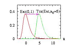 The class Translate.hpp allows you to translate the density
function by x0.
The class Translate.hpp allows you to translate the density
function by x0.
x → x+x0
then the new instance Translate(&distribution,x0)
can be used at an usual distribution.
In addition to the general
syntax, we have:
| void setParameter(Distribution* d, double x0); |
|
where Distribution* is the address of the distribution to transform. |
| void refresh( ); |
|
if the distribution (Extreme in our example) has changed, you should refresh the class. This is not done automatically because it is very time-consuming to check it at each call of ran( ). Moreover the call of refresh() calls the refresh( ) function of the distribution given as parameter. |
The program to generate the figure above could be:
// Example Translate1.cpp download
//
#include "LOPOR.hpp"
using namespace LOPOR;

int main( )
{
    try
    {
        Extreme Ext;
        Ext.setParameter(0,1);
        Translate trans;
        trans.setParameter(&Ext,5);

        // vecX={-3, -2.99, -2.98,…, 12.99, 13}
        std::vector<double> vecX(vec_create(1601,-3.,0.01));

        // to create the figure above:
        // print in file "Translate1.res", the vectors:
        // i           vecX   density(Extreme) density(Translate)
        // 0             -3   3.80054e-08              0
        // 1          -2.99   4.59514e-08              0
        // 2          -2.98         …               …
        vec_print("Translate1.res",vecX,Ext.densityVector(vecX),
                  trans.densityVector(vecX));

        // print 10 random numbers
        vec_print(trans.ranVector(10),"ran ");
    }
    catch (const LOPOR::Error& error) { error.information( ); }
    return 0;
}
And the program will create the file "Translate1.res" used to plot the figure above and print on the screen:
#   i=      ran
     0        7.26301
     1        3.59437
     2        4.54731
     3        4.75202
     4        5.19198
     5        5.51945
     6        4.84831
     7        5.87925
     8        6.13524
     9        5.24774
You can construct a new distribution class fairly easily. The only necessary function should be the ran( ) function or the density( ) function. If you also define some other functions like the cumulative( ) function, you will also be able to use the Transformations-Sum classes. If you do not know a simple way to produce the random numbers from this distribution, you should use one of the rejection methods: Hasting or HeatBath. We will present now some possibilities.
In this section we will show how we have constructed
the Exponential class. The
density mass function is :
f(x)= exp(− x/a)/a
It consists in one declaration file Exponential.hpp and one other file
Exponential.cpp.
// download Exponential.hpp
#ifndef EXPONENTIAL_HPP
#define EXPONENTIAL_HPP

#include "Distribution.hpp"

namespace LOPOR
{
class Exponential : public Distribution{
    public:
        Exponential( );
        ~Exponential( ){};
        virtual void                setParameter(const double& a) ;
        virtual void                setParameters(const std::vector <double> & parameters);
        virtual double              density     (const double& x) ;
        virtual double              cumulative  (const double& x) ;
        virtual double              mean        ( )                ;
        virtual double              mode        ( )                ;
        virtual double              variance    ( )                ;
        virtual double              ran_fc(const double& ran)     ;
         virtual Distribution*       clone( )                       ;
        virtual std::vector <double>  moments(const std::vector<double > & vecX);
        virtual std::vector <double>  mle(const std::vector<double > & vecX);
        virtual std::vector <double>  fit_cum(const double x
                                            , std::vector<double > & coeff);
        virtual std::vector <double>  fit_den(const double x
                                            , std::vector<double > & coeff);

    private:
                double              A;

};
} // !namespace LOPOR

#endif /* EXPONENTIAL_HPP */
and the Exponential.cpp file:
// download Exponential.cpp
#include "Error.hpp"
#include "Vector.hpp"
#include "Exponential.hpp"

LOPOR::Exponential::Exponential( )
{
    type="double";
    name="Exponential";
    fit_keep_den_LM=c2v <int> ( );
    fit_keep_cum_LM=c2v <int> ( );
    setParameter(1);
}

void LOPOR::Exponential::setParameters(const std::vector <double> & parameters)
{
    int temp=1;
    if(parameters.size( ) != temp) throw Error("LOPOR:"+name
            +":setParameter(vector <double>  parameters): parameters should have "
            +c2s(temp)
            +" elements or parameters.size( )="+c2s(parameters.size( )));
    setParameter(parameters[0]);
}

void LOPOR::Exponential::setParameter(const double& a)
{
    Parameters=c2v(a);
    A=a;
    if(a < 0) throw Error(information( )+"::setParameter( ) = >  The variable:"
            + c2s(a) +" must be  > = 0");
    Ftot=1;
}

double LOPOR::Exponential::density(const double& x)
{
    if(x < 0) return 0.;
    return exp(-x/A)/A;
}

double LOPOR::Exponential::cumulative(const double& x)
{
    if(x < 0) return 0.;
    return 1.-exp(-x/A);
}

double LOPOR::Exponential::mean( )
{
    return A;
}

double LOPOR::Exponential::mode( )
{
    return 0.;
}

double LOPOR::Exponential::variance( )
{
    return A*A;
}

double LOPOR::Exponential::ran_fc(const double& ran)
{
    return -A*log(1-ran);
}

LOPOR::Distribution* LOPOR::Exponential::clone( )
{
    Exponential* clone = new Exponential( );
    *clone = *this;
    return clone;
}

std::vector <double>  LOPOR::Exponential::moments
            (const std::vector<double > & vecX)
{
    if(vecX.size( ) ==0) throw Error("LOPOR::"
                       +name+"::moments(vecX) : no data in VecX");
    double mean=vec_mean(vecX);
    std::vector <double>  vec=c2v<double > (mean);
    setParameters(vec);
    return vec;
}


std::vector <double>  LOPOR::Exponential::mle(const std::vector<double > & vecX)
{
    if(vecX.size( ) ==0) throw Error("LOPOR::"+name+"::mle(vecX) : no data in VecX");
    std::vector <double>  vec=c2v<double > (vec_mean(vecX));
    setParameters(vec);
    return vec;
}

std::vector <double>  LOPOR::Exponential::fit_cum(const double x,
                    std::vector<double > & coeff)
{
    if(coeff.size( )!= Parameters.size( )) throw Error("LOPOR::"+name
            +"::fit: the coeff.size( )="+c2s(coeff.size( ))
            +"!= nb of parameters="+c2s(Parameters.size( )));

    if(coeff!=Parameters) setParameters(coeff);

    // Levemberg-Marquardt: derivatives+function
    std::vector <double>  lm(coeff.size( )+2);
    lm[0]=-(x/(Power(A,2)*Power("E",x/A))); // derivative by coeff[0]
    lm[1]= 1/(A*Power("E",x/A)); // derivative by x
    lm[2]=cumulative(x);     // function
    return lm;
}

std::vector <double>  LOPOR::Exponential::fit_den(const double x,
                    std::vector<double > & coeff)
{
    if(coeff.size( )!= Parameters.size( )) throw Error("LOPOR::"+name
            +"::fit: the coeff.size( )="+c2s(coeff.size( ))
            +"!= nb of parameters="+c2s(Parameters.size( )));

    if(coeff!=Parameters) setParameters(coeff);

    // Levemberg-Marquardt: derivatives+density
    std::vector <double>  lm(coeff.size( )+2);
    lm[0]=(-A + x)/Power(A,2)*density(x); // derivative by coeff[0]
    lm[1]= -(1/A)*density(x); // derivative by x
    lm[2]=density(x);     // density
    return lm;
}
Explanations:
The other functions defined in General Syntax Distribution
are available automatically.
We have defined the function ran_fc and all the other
ran functions of the General Syntax Distribution: ran( ),
ranVector, ranVectorLH,
are available automatically. However for some distributions it is impossible to
inverse and solve the equation F-1(x)=y. Two choices:
The discrete distribution classes follow the same procedure as the continuous distributions. There are three points worth to be noted :
The library uses distributions to exchange information between elements,
therefore it is sometimes better to have a distribution
instead of a function.
The class FunctionDistribution
provides it. Only the density function of the general
syntax is defined, and in addition we have:
| void setParameter(double func(const double& x)) |
|
define the function |
An example of program:
// Example FunctionDistribution.cpp

#include "LOPOR.hpp"
using namespace LOPOR;

double func(const double& x) { return 2.*x; }

int main( )
{
    try
    {
        FunctionDistribution function;
        function.setParameter(func);
        print(function.density(3.));
    }
    catch (const Error& error) { error.information( ); }
    return 0;
}
And the output of this program is:
6
 The class Hasting.hpp allows you to produce a random number
generator for any
density function. It is not as good as the HeatBath
but a little bit easier to implement. For an introduction and
a comparison with the HeatBath method see
[Loison2004].
The main point is to simulate a complicated distribution
d1 using another distribution d2
easier to simulate, using a kind of rejection method.
Contrary to the HeatBath the d2
function f2 is not
necessarily bigger than the d1 function
f1. Therefore
any distribution d2 is a possible candidate.
However the closest f2 is of f1 the
more efficient the algorithm will be. The only restriction
for the choice of f2 is that it must not be zero
if f1 is not zero.
The class Hasting.hpp allows you to produce a random number
generator for any
density function. It is not as good as the HeatBath
but a little bit easier to implement. For an introduction and
a comparison with the HeatBath method see
[Loison2004].
The main point is to simulate a complicated distribution
d1 using another distribution d2
easier to simulate, using a kind of rejection method.
Contrary to the HeatBath the d2
function f2 is not
necessarily bigger than the d1 function
f1. Therefore
any distribution d2 is a possible candidate.
However the closest f2 is of f1 the
more efficient the algorithm will be. The only restriction
for the choice of f2 is that it must not be zero
if f1 is not zero.
The new instance
Hasting(&distribution1,&distribution2)
can be used at an usual distribution. This method in combination with
the StepFunction class is the fastest method if the
ran_fc( ) of the distribution
d1 is unknown
[Loison2004].
If the distribution function f2 is constant, we get the
Metropolis algorithm.
If the distribution d2 is
the UniformDelta
distribution we
get the Restricted Metropolis procedure. This last procedure
must be used when the form of the distribution d1
is too wide to define an efficient function f2
[Loison2004].
In addition to the general
syntax, we have:
| void setParameter(Distribution* d1, Distribution* d2, double xini); |
|
The Distribution* d1
is the address of the distribution that we are interested in. |
|
double successPerCent( ); |
|
return the % of success of the calls for ran( ) and ranVector( ) functions of the new Hasting instance. |
| void refresh( ); |
|
if the distribution (Gamma in our example) has changed, you should refresh the class. This is not done automatically because it is very time-consuming to check it at each all of ran( ) call. Moreover the call of refresh() calls the refresh( ) function of the distributions given as parameter. |
Fit
All fit functions described in Fit are accessible.
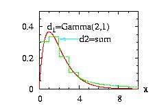
The program to
generate the figure above could be:
// Example Hasting1.cpp download
//
// Objective: have a random number generator for
// the Gamma class  if we admit that we do not know
// how to implement it directly.
//
#include "LOPOR.hpp"
using namespace LOPOR;

int main( )
{
    try
    {
        // The class which we do not know (!) the ran( ) function
        Gamma Gam;
        Gam.setParameter(2,1);

        // Construct of the distribution to simulate Gamma
        // The density should be as near as possible of the
        // distribution studied (here Gamma)
        //
        // 1. For x between 0 and 4: a StepFunction with 5-1=4 steps
        StepFunction Ste;
        Ste.setParameter(&Gam,0,4,5);

        // 2. For x > 4 : A Pareto fc: the class Interval
        // with border=2 (last parameter) : [4,+oo[
        Pareto Par;
        Par.setParameter(1,16*Gam.density(4));
        Interval Int;
        Int.setParameter(&Par,4,11,2);

        // 3. Sum of the two functions:
        Sum sum;
        sum.setParameter(c2v <Distribution*> (&Ste,&Int));

        // The instance Has can be used as an instance of the Gamma class
        Hasting Has;
        Has.setParameter(&Gam,&sum,1);

        // vecX={0, 9.99, 10}
        std::vector<double> vecX(vec_create(1001,0.,0.01));

        // to create the figure above:
        // print in file "Hasting1.res", the vectors:
        // i   x  Hasting=Gamma  Sum
        vec_print("Hasting1.res",vecX,Has.densityVector(vecX),
                                 sum.densityVector(vecX));

        // print 10 random numbers from the Gamma distribution
        // through the Hasting instance
        vec_print(Has.ranVector(10),"ran for Gamma ");
    }
    catch (const Error& error) { error.information( ); }
    return 0;
}
And the program will create the file "Hasting1.res" used to plot the figure above) and print on the screen:
#   i=      ran for Gamma
     0        2.74109
     1        7.38208
     2        4.53815
     3        0.61207
     4        0.68343
     5        1.38852
     6        4.41928
     7        4.99977
     8        1.70519
     9        1.70519
 The class HeatBath.hpp allows you to produce a random number
generator for any
density function. This method is known generally as the
"rejection method". It is a little better than the Hasting
procedure,
but a little bit more difficult to implement. For an introduction and
a comparison with the Hasting method see
[Loison2004].
The main point is to simulate a complicated distribution
d1 using another distribution d2
which is easier to simulate, using a kind of rejection method.
Contrary to the Hasting method the d2
function f2 must be
bigger than the d1 function
f1.
The closest f2 is of f1 the
more efficient the algorithm will be.
Then the new instance,
HeatBath(&distribution1,&distribution2),
can be used at an usual distribution. This method in combination with
the StepFunction class is the fastest method if the
ran_fc( ) of the distribution
d1is unknown
[Loison2004].
The class HeatBath.hpp allows you to produce a random number
generator for any
density function. This method is known generally as the
"rejection method". It is a little better than the Hasting
procedure,
but a little bit more difficult to implement. For an introduction and
a comparison with the Hasting method see
[Loison2004].
The main point is to simulate a complicated distribution
d1 using another distribution d2
which is easier to simulate, using a kind of rejection method.
Contrary to the Hasting method the d2
function f2 must be
bigger than the d1 function
f1.
The closest f2 is of f1 the
more efficient the algorithm will be.
Then the new instance,
HeatBath(&distribution1,&distribution2),
can be used at an usual distribution. This method in combination with
the StepFunction class is the fastest method if the
ran_fc( ) of the distribution
d1is unknown
[Loison2004].
In addition to the general
syntax, we have:
| void setParameter(Distribution* d1, Distribution* d2); |
|
The Distribution* d1
is the address of the distribution that we are interested in. |
|
double successPerCent( ); |
|
return the % of success of the calls for ran( ) and ranVector( ) functions of the new HeatBath instance. |
| void refresh( ); |
|
if the distribution (Gamma in our example) has changed, you should refresh the class. This is not done automatically because it is very time-consuming to check it at each all of ran( ) call. Moreover the call of refresh() calls the refresh( ) function of the distributions given as parameter. |
Fit
All fit functions described in Fit are accessible.
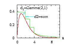
The program to
generate the figure above could be:
// Example HeatBath1.cpp download
//
// Objective: have a random number generator for
// the Gamma class  if we admit that we do not know
// how to implement it directly.
//
#include "LOPOR.hpp"
using namespace LOPOR;

int main( )
{
    try
    {
        // The class which we do not know (!) the ran( ) function
        Gamma Gam;
        Gam.setParameter(2,1);

        // Construct of the distribution to simulate Gamma
        // The density should be as near as possible of the
        // distribution studied (here Gamma)
        //
        // 1. For x between 0 and 4: a StepFunction with 5-1=4 steps
        //    "Maximum": the step function is higher that the Gamma
        StepFunction Ste;
        Ste.setParameter(&Gam,0,4,5,"Maximum");

        // 2. For x > 4 : A Pareto fc: the class Interval
        // with border=2 (last parameter) : [4,+oo[
        Pareto Par;
        Par.setParameter(1,16*Gam.density(4));
        Interval Int;
        Int.setParameter(&Par,4,11,2);

        // 3. Sum of the two functions:
        Sum sum;
        sum.setParameter(c2v <Distribution*> (&Ste,&Int));

        // The instance HB can be used as an instance of the Gamma class
        HeatBath HB;
        HB.setParameter(&Gam,&sum);

        // vecX={0, 9.99, 10}
        std::vector<double> vecX(vec_create(1001,0.,0.01));

        // to create the figure above:
        // print in file "HeatBath1.res", the vectors:
        // i   x  HeatBath=Gamma  Sum
        vec_print("HeatBath1.res",vecX,HB.densityVector(vecX),
                                 sum.densityVector(vecX));

        // print 10 random numbers from the Gamma distribution
        // through the HeatBath instance
        vec_print(HB.ranVector(10),"ran for Gamma ");
    }
    catch (const Error& error) { error.information( ); }
    return 0;
}
And the program will create the file "Hasting1.res" used to plot the figure above and print on the screen:
#   i=      ran for Gamma
     0        1.95226
     1       0.667258
     2       0.324795
     3        1.43791
     4       0.685709
     5       0.616973
     6        3.57849
     7       0.563728
     8        2.43355
     9        2.14097
The MetropolisRestricted is related to the Hasting class,
however it is not based on a distribution. It allow the users
to generate random numbers from a multivariate distribution g. It consists
to create a Markov chain updating each variables consecutively. This is done at follow:
1. From a configuration {x0,x1,…} create a new configuration:
{x0new,x1,…} using
x0new=x0 ± δ0
with delta fixed at the beginning of the simulation.
2. Accept this new configuration with the probability g(new)/g(old)
Then try to updated the second variable, then the third, …
For more information see [Loison2004].
One flaw of this method is that the random number will be correlated and
a careful analysis should be done to measure the correlation using
the Autocorrelation function. An example is given
here. Moreover we need a certain number of step at the
beginning of the procedure to reach a configuration in equilibrium.
| void setParameter(double function(const vector<double>&), vector<double> x_ini,vector<double> delta_ini,int MC_eq=1000,int keep_data=1 ); |
|
The function we are interested in. |
|
vector<double> successPerCent( ); |
|
return the % of success of the procedure for each variable. |
|
vector<double> ran( ); |
|
return a vector composed of random number for each variable. |
|
vector<vector<double> > ranVector(int MC); |
|
return MC vectors, each composed of random numbers for each variable. |
An example of program can be found here.
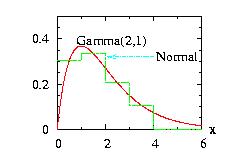
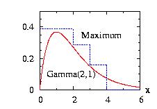
The StepFunction class is based on the Histogram class.
The user must give the {xi} coordinates and
the distribution d to be approximated, the class calculate the
probabilities {pi}. There are two options: the
StepFunction function f can be always bigger than the
distribution function, or the {pi} are calculated
using the middle of each [xi,xi+1]
interval. This class is very powerful in combination
with the HeatBath and the
Hasting classes. If the number of
step increases the function will be approximated better but
the time consumption will not necessary decrease because
more memory is needed to store the data
[Loison2004].
Hundreds steps of should be a maximum.
| class: | StepFunction.hpp |
| density: |
two choices:
|
| restrictions: |
n ≥ 2 pi ≥ 0 and at least one pi ≠ 0, there are n−1 probabilities pi xi < xi+1, there are n values xi |
| domain: | x0 ≤ x ≤ xn−1 |
| cumulative: | |
| mean: | |
| mode: | no closed form |
| variance: |
In addition to the general syntax, we have:
| void setParameter( Distribution* d, vector <double> x, string name_type, vector <double> vecMax); |
|
d is the distribution to
approximate |
| void setParameter( Distribution* d, double xmin, double xmax, int n, string name_type, vector <double> vecMax); |
|
The difference between the setParameter above is that the vector x is calculated by the class. You should give the xminimum, the xmaximum and the number of interval+1= n |
| vector <double> get_X( ) |
|
return the vector x |
| void change_X(vector <double> x) |
|
if the vector x calculated by the class does not fit your needs. Similar as redoing a setParameter( ). |
| vector <double> get_P( ) |
|
return the vector p (probabilities) |
| void change_P(vector <double> p) |
|
if the vector p calculated by the class does not fit your needs. |
| void normalize( ) |
|
Normalize the distribution, i.e. ∫x[o]x[end] density = 1 |
| int get_i ( double x ) |
|
return the number of the interval (0 to n−1) corresponding to the value x. |
|
vector <double> E.ranVectorLH(int n); double E.ran_fc(double y); |
|
not defined |
Fit No fit functions described in Fit are accessible.
Programs to generate the figures above are Hasting1.cpp for the first figure and HeatBath1.cpp for the second figure.
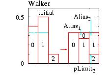 The class Walker.hpp is not based on a Distribution
class. You should use only the functions listed below.
This class is used in some distribution classes to
accelerate the simulations.
Walker's alias method handles in an economic way which new
state to choose among n possibilities.
The probabilities pi for a new state i
are stored in n different boxes of equal
height ∑pi/n.
Walker's construction has in each box only
one or two different probabilities. For an example with
n=3 see the figure. Before the simulation
starts one must have calculated and stored the probabilities
pLimiti which divides each box i. The upper
states in each box must also be stored in an array. These
states as ``subtenants'' have an ``alias'' whereas the
lower ones have the box number as correct address for the
state i.
The implementation has the following steps:
The class Walker.hpp is not based on a Distribution
class. You should use only the functions listed below.
This class is used in some distribution classes to
accelerate the simulations.
Walker's alias method handles in an economic way which new
state to choose among n possibilities.
The probabilities pi for a new state i
are stored in n different boxes of equal
height ∑pi/n.
Walker's construction has in each box only
one or two different probabilities. For an example with
n=3 see the figure. Before the simulation
starts one must have calculated and stored the probabilities
pLimiti which divides each box i. The upper
states in each box must also be stored in an array. These
states as ``subtenants'' have an ``alias'' whereas the
lower ones have the box number as correct address for the
state i.
The implementation has the following steps:
The time consumption is therefore independent on the number of states. The only limitation is the memory needed to store the arrays. The method to generate the arrays can be found in the Peterson1979. The syntax :
| void setParameter(vector <double> probabilities); |
|
where probabilities={p0,p1, …,pn−1} |
| double ran( ); |
|
return a random number following the probabilities distribution |
| double ran(double ra ); |
|
return a random number following the probabilities distribution and a new random number (uniform distribution between 0 and 1) ra which is calculated during the walker procedure |
| vector <double> ranVector(int n); |
|
return n random numbers following the probabilities distribution |
| vector <double> ranVector(int n, vector <double> ranVec); |
|
return n random numbers following the probabilities distribution and n random numbers (uniform distribution between 0 and 1) ranVec which are calculated during the walker procedure |
| vector <double> ranVectorLH(int n); |
|
return n random numbers following the probabilities distribution, using the Latin Hypercube sampling. Give a better result than ranVector(n), but you must be cautious when using it: all the random numbers must be used to calculate the integrals. |
| vector <double> ranVectorLH(int n, vector <double> ranVec); |
|
Same as previous line, but return also n random numbers (uniform distribution between 0 and 1) ranVec which are calculated during the walker procedure |
| vector <double> cumulativeVector(double Ftot); |
|
return the cumulative for all {i} as
a vector: cumulativeVector
={F0,
F1, … ,Fn−1}
={p0/Ftot,(p0+p1)/Ftot,
… ,1}. |
The library uses distributions to exchange information between elements,
therefore it is sometimes better to have a distribution
instead of a function. We have defined several function on the form of
a Distribution.
If you want to transform
a function in a distribution form you should use the class
FunctionDistribution defined thereafter.
Only the density of the
function is defined. You cannot use directly an instance of the distribution
function with the ran() function. If you need a random generator you should
use in combination the Hasting class or the
HeatBath class.
For the predefined distribution functions
(Exponential_fc ,
Laguerre_fc, …) the
fit_den function is defined and therefore you can use
the Levemberg-Marquardt method to fit parameters using
the Fit::LeastSquares_LM_den static function.
The class FunctionDistribution
transform a static function in an instance of
Distribution.
Only the density function of the general
syntax is defined, and in addition we have:
| void setParameter(double func(const double& x)) |
|
define the function |
An example of program:
// Example FunctionDistribution.cpp

#include "LOPOR.hpp"
using namespace LOPOR;

double func(const double& x) { return 2.*x; }

int main( )
{
    try
    {
        FunctionDistribution function;
        function.setParameter(func);
        print(function.density(3.));
    }
    catch (const Error& error) { error.information( ); }
    return 0;
}
And the output of this program is:
6
The Exponential_fc class defined the function
f(x) = B e A x
Only the density function of the general
syntax is defined, and in addition we have:
| void setParameter(A,B) |
|
void
setParameters(vector<double> parameters)
|
|
with parameters={A,B} |
The fit function Fit::LeastSquares_LM_den can be used with this class.
The Laguerre_fc class defined the function
f(x) = e−x/2 ∑n=0N an Ln(x)
Ln(x) = ex/n! dn/dxn (Xn e−x)
Be aware that we have add the exponential factor in front of the standard
Laguerre polynomial functions. We have:
L0(x) = 1
L1(x) = 1 − x
L2(x) = 1 − 2x + x2/2
Ln(x) = (2n − 1 − x)/n Ln−1
− (n − 1)/n Ln−2
Only the density function of the general
syntax is defined, and in addition we have:
|
void
setParameters(vector<double> parameters)
|
|
parameters={a0,a1,…} |
The fit function Fit::LeastSquares_LM_den
can be used with this class. Example of program:
Laguerre_fc laguerre; // define instance
laguerre.setParameters(c2v(0.5,0.2,1.)); // three first Laguerre fc
std::vector<double> X,Y; // create data for fit
for(double x=0; x<10; x += 0.1)
{
X.push_back(x);
Y.push_back(laguerre.density(x));
}
print("data from:",laguerre.information()); // display information
laguerre.setParameters(c2v(0.7,0.4,0.9)); // change parameters
print("before fit:",laguerre.information());
Fit::LeastSquares_LM_den(&laguerre,X,Y); // Fit
print("after fit:",laguerre.information());
And the output is:
data from: LOPOR::Laguerre_fc(0.5,0.2,1)
before fit: LOPOR::Laguerre_fc(0.7,0.4,0.9)
after fit: LOPOR::Laguerre_fc(0.5,0.2,1)
The Linear_fc class defined the function
f(x) = A + B * x
Only the density function of the general
syntax is defined, and in addition we have:
| void setParameter(A,B) |
|
void
setParameters(vector<double> parameters)
|
|
with parameters={A,B} |
The fit function Fit::LeastSquares_LM_den can be used with this class.
The Polynome_fc class defined the function
f(x) = ∑i=0N ai xi
f(x) = a0 + a1 x + a2 x2 + …
Only the density function of the general
syntax is defined, and in addition we have:
|
void
setParameters(vector<double> parameters) |
|
parameters={a0,a1,…} |
|
void setParameter(int degree) |
|
f(x) = 1 + x + x2 + … + xdegree |
Example:
Polynome_fc polynome;
polynome.setParameters(c2v(1.,1.5,1.));
print(polynome.information());
And the output is:
LOPOR::Polynome_fc( 1*x^0 + 1.5*x^1 + 1 x^2 )
The fit function Fit::LeastSquares_Linear_den
can be used with this class. We give thereafter the function
fit_den_linear used by this Fit function. It returns
a vector {x0,x1,…}
std::vector<double> LOPOR::Polynome_fc::fit_den_linear(const double x)
{

    std::vector<double> lm(Parameters.size());
	if(Parameters.size()>=1) lm[0]=1;
	for(int i=1; i<Parameters.size(); ++i)
		lm[i]=lm[i-1]*x;
	return lm;
}
There are three main methods for generating multivariate random
vectors of n elements each.
The first is the acceptance/rejection method, the second
the conditional distribution, and the third the partially-specified-properties
transformation.
The acceptance/rejection method is mainly use in one dimension. For example
the class StepFunction use this method. There
are several problems:
First we need to know the exact form of the distribution
function f and not only the correlation matrix.
Second we have to define a function g which is always bigger
than the f, g ≥ f, that we know the inverse of the cumulative function
G−1. It is usually very difficult to find a correct function,
in particular if f has a lot of maximum and if we are in high dimension.
We can use the StepFunction
in two dimension [Loison2004] but in higher dimension
the memory needed increases exponentially.
The second method is to produce iteratively the elements: the first without
constraint, the second random number with the constraint with the first
distribution, the third with the constraint on the first and the
second distribution, … This procedure becomes very cumbersome
and almost impracticable for all but the normal distribution
NormalMulti and
NormalMultiPCA.
The third method is used by the NORTA algorithm and
is very powerful.
The class NormalMulti.hpp is not based on the Distribution
class.
The probability density function is:
f(x) = (2 π)−n/2 |Σ|1/2
exp[
− (x − μ)T Σ−1 (x − μ) / 2 )
]
with Σ is the variance-covariance matrix,
x={x1,x2,…xn} and
μ={μ1,μ2,…μn}
are a two vectors of n elements. T means transposed
A way to generate the vector x is to construct a vector z of n Normal random numbers
and to use:
x = MT z + μ
with the condition that MT M = Σ.
We use this method with a Cholesky
decomposition which gives the matrix
MT under the form of a lower diagonal matrix with 0
on the upper diagonal part. The class NormalMulti.hpp
provides these functions:
| void setParameter(vector<double> μ, vector<vector<double> > Σ) | ||||||||||||||||||||
|
μ = {μ1, μ2, …, μn}
|
||||||||||||||||||||
|
void setParameter(vector<double> μ, vector<double> σ, vector<vector<double> > Σ') void setParameter(vector<vector<double> > Σ') |
||||||||||||||||||||
|
μ = {μ1, μ2, …, μn}, if not given all μi=0
|
||||||||||||||||||||
| vector<double> ran( ) | ||||||||||||||||||||
|
return a vector of n normal random numbers correlated through the correlation matrix Σ |
||||||||||||||||||||
| vector<vector<double> > ranVector(int L ) | ||||||||||||||||||||
|
return a matrix of L vectors of n normal random numbers correlated through the correlation matrix Σ |
Example of program:
// Example NormalMulti.cpp
// call L*2 normal random numbers correlated
// plot the histogram to check that both variables
// follows a Normal distribution

#include "LOPOR.hpp"
using namespace LOPOR;

int main( )
{
    try
    {
        // correlation matrix Sigma':
        std::vector<std::vector<double> > correlations;
        correlations=c2m(c2v(1.,0.6),c2v(0.6,1.));

        // mean vector
        std::vector<double> mean(c2v(1.,2.));

        // sigma vector
        std::vector<double> sigma(c2v(1.,2.));

        // create instance
        NormalMulti normalMulti;
        normalMulti.setParameter(mean,sigma,correlations);

        // results
        std::vector<std::vector<double> > matrix_res;

        // matrix_res={ {a0,b0}, {a1,b1}, …, {aL,bL} }
        matrix_res=normalMulti.ranVector(100000);

        // matrix_res={ {a0,a1,a2…,aL} , {b0,b1,b2,…,bL} }
        matrix_res=matrix_transposed(matrix_res);

        // check correlation
        print("correlations a.b=",
                vec_mean(vec_multiply(
                        vec_add(matrix_res[0],-mean[0]),
                        vec_add(matrix_res[1],-mean[1])
                        ))
                , ", exact=",correlations[0][1]*sigma[0]*sigma[1]);

        // Construct histogram on [-5:10] with 100 bins with normalization
        // and print in files
        vec_histogram_print("NormalMulti0.res",matrix_res[0],-5,10,100);
        vec_histogram_print("NormalMulti1.res",matrix_res[1],-5,10,100);
    }
    catch (const Error& error) { error.information( ); }
    return 0;
And the output is:
correlations a.b= 1.18792 , exact= 1.2
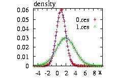
Columns 3 as function of the column 2 of the files
"NormalMulti0.res" and "NormalMulti1.res" and the densities
e-(x-mean)2/(2 σ2)
to check the results.
The class NormalMultiPCA.hpp is not based on the Distribution
class.
The probability density function is:
f(x) = (2 π)−n/2 |Σ|1/2
exp[
− (x − μ)T Σ−1 (x − μ) / 2 )
]
with Σ is the variance-covariance matrix,
x={x1,x2,…xn} and
μ={μ1,μ2,…μn}
are a two vectors of n elements. T means transposed
We first diagonalize Σ = Γ Λ ΓT
with Λ a diagonal matrix of the λi
eigenvalues on the diagonal. We have the properties that
ΓT=Γ−1.
Then we construct the matrix Λ', a diagonal matrix
with (λi)½ on the diagonal.
Second we generate a vector z of n Normal
random numbers and we get
the new correlated random numbers using Γ Λ' z.
The interest of this method compared to the
previous one is that we are able to
speed up the procedure if some variables are strongly correlated. In the
example below, NormalMultiPCA.cpp,
we are able to use only two random numbers to obtain "three" random numbers,
loosing only 1% of precision.
The class NormalMultiPCA.hpp
provides these functions and variables:
| void setParameter(vector<double> μ, vector<vector<double> > Σ, double percent=1) | ||||||||||||||||||||
|
μ = {μ1, μ2, …, μn}
|
||||||||||||||||||||
|
void setParameter(vector<double> μ, vector<double> σ, vector<vector<double> > Σ', double percent) void setParameter(vector<vector<double> > Σ', double percent) |
||||||||||||||||||||
|
μ = {μ1, μ2, …, μn}, if omitted ={0,0,…}
|
||||||||||||||||||||
| vector<double> ran( ) | ||||||||||||||||||||
|
return a vector of n normal random numbers correlated through the correlation matrix Σ |
||||||||||||||||||||
| vector<vector<double> > ranVector(int L ) | ||||||||||||||||||||
|
return a matrix of L vectors of n normal random numbers correlated through the correlation matrix Σ |
||||||||||||||||||||
|
int Np vector<double> eigenvalues vector<vector<double> > eigenvectorsTVector |
||||||||||||||||||||
|
Np = number of non correlated normal random numbers generated |
Example of program:
// Example NormalMultiPCA.cpp
// Call L*3 normal random numbers correlated using PCA
// Plot the histogram to check that both variables
//    follows a Normal distribution
// Check if we use only 2 non correlated normal
//    random numbers to create 3 correlated random numbers

#include "LOPOR.hpp"
using namespace LOPOR;

int main( )
{
    try
    {
        // correlation matrix Sigma':
        // matrix : strong correlation between the
        // second and third component
        // | 1   0.05   0.05 |
        // | 0.05   1   0.95 |
        // | 0.05  0.95   1  |
        std::vector<std::vector<double> > correlations=
        c2m( c2v(1.,0.05,0.05), c2v(0.05,1.,0.95), c2v(0.05,0.95,1.));

        // mean vector
        std::vector<double> mean(c2v(1.,2.,3.));

        // sigma vector
        std::vector<double> sigma(c2v(1.,2.,1.));

        // create instance
        NormalMultiPCA normalMultiPCA;

    // ------------------ I -------------------
        // percent omitted => =100% : we use 3 random numbers
        normalMultiPCA.setParameter(mean,sigma,correlations);

        // check that Np=3 (use 3 random numbers)
        // and plot eigenvalues
        print("Np=",normalMultiPCA.Np);
        vec_print_1(normalMultiPCA.eigenvalues,"eigenvalues=");
        vec_print_1(vec_normalize(normalMultiPCA.eigenvalues),"normalized =");
        vec_print_1(vec_cumulative_histo(normalMultiPCA.eigenvalues),"%          =");
        print( );

        // results
        std::vector<std::vector<double> > matrix_res;

        // matrix_res={ {a0,b0,c0}, {a1,b1,c1}, …, {aL,bL,cL} }
        matrix_res=normalMultiPCA.ranVector(1000000);

        // matrix_res={ {a0,a1,a2…,aL} , {b0,b1,b2,…,bL} , {c0,c1,c2…,cL} }
        matrix_res=matrix_transposed(matrix_res);

        // check correlation
        print("correlations a.b=",
                vec_mean(vec_multiply(
                        vec_add(matrix_res[0],-mean[0]),
                        vec_add(matrix_res[1],-mean[1])
                        ))
                , ", exact=",correlations[0][1]*sigma[0]*sigma[1]);

        print("correlations a.c=",
                vec_mean(vec_multiply(
                        vec_add(matrix_res[0],-mean[0]),
                        vec_add(matrix_res[2],-mean[2])
                        ))
                , ", exact=",correlations[0][2]*sigma[0]*sigma[2]);

        print("correlations b.c=",
                vec_mean(vec_multiply(
                        vec_add(matrix_res[1],-mean[1]),
                        vec_add(matrix_res[2],-mean[2])
                        ))
                , ", exact=",correlations[1][2]*sigma[1]*sigma[2]);
        print( );

        // Construct histogram on [-5:10] with 100 bins with normalization
        // and print in files
        vec_histogram_print("NormalMultiPCA0.res",matrix_res[0],-5,10,100);
        vec_histogram_print("NormalMultiPCA1.res",matrix_res[1],-5,10,100);
        vec_histogram_print("NormalMultiPCA2.res",matrix_res[2],-5,10,100);

    // ------------------ II -------------------
        // 0.98=98 %percent : we use 2 random numbers
        normalMultiPCA.setParameter(mean,sigma,correlations,0.98);
        // We can also impose normalMultiPCA.Np=2

        // check that Np=2 (use 2 random numbers)
        // and plot eigenvalues
        print("Np=",normalMultiPCA.Np);
        vec_print_1(normalMultiPCA.eigenvalues,"eigenvalues=");
        vec_print_1(vec_normalize(normalMultiPCA.eigenvalues),"normalized =");
        vec_print_1(vec_cumulative_histo(normalMultiPCA.eigenvalues),"%          =");
        print( );

        // matrix_res={ {a0,b0,c0}, {a1,b1,c1}, …, {aL,bL,cL} }
        matrix_res=normalMultiPCA.ranVector(1000000);

        // matrix_res={ {a0,a1,a2…,aL} , {b0,b1,b2,…,bL} , {c0,c1,c2…,cL} }
        matrix_res=matrix_transposed(matrix_res);

        // check correlation
        print("correlations a.b=",
                vec_mean(vec_multiply(
                        vec_add(matrix_res[0],-mean[0]),
                        vec_add(matrix_res[1],-mean[1])
                        ))
                , ", exact=",correlations[0][1]*sigma[0]*sigma[1]);

        print("correlations a.c=",
                vec_mean(vec_multiply(
                        vec_add(matrix_res[0],-mean[0]),
                        vec_add(matrix_res[2],-mean[2])
                        ))
                , ", exact=",correlations[0][2]*sigma[0]*sigma[2]);

        print("correlations b.c=",
                vec_mean(vec_multiply(
                        vec_add(matrix_res[1],-mean[1]),
                        vec_add(matrix_res[2],-mean[2])
                        ))
                , ", exact=",correlations[1][2]*sigma[1]*sigma[2]);
        print( );

        // Construct histogram on [-5:10] with 100 bins with normalization
        // and print in files
        vec_histogram_print("NormalMultiPCA3.res",matrix_res[0],-5,10,100);
        vec_histogram_print("NormalMultiPCA4.res",matrix_res[1],-5,10,100);
        vec_histogram_print("NormalMultiPCA5.res",matrix_res[2],-5,10,100);
    }
    catch (const Error& error) { error.information( ); }
    return 0;
And the output is:
Np= 3
eigenvalues= 4.92393 0.996817 0.0792542
normalized = 0.820655 0.166136 0.013209
%          = 0.820655 0.986791 1

correlations a.b= 0.101926 , exact= 0.1
correlations a.c= 0.0507717 , exact= 0.05
correlations b.c= 1.89816 , exact= 1.9

Np= 2
eigenvalues= 4.92393 0.996817 0.0792542
normalized = 0.820655 0.166136 0.013209
%          = 0.820655 0.986791 1

correlations a.b= 0.101037 , exact= 0.1
correlations a.c= 0.0506329 , exact= 0.05
correlations b.c= 1.92847 , exact= 1.9
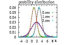
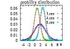
Column 3 as function of the column 2 of the files
"NormalMulti0.res", "NormalMulti1.res", and "NormalMulti2.res"
for the first plot.
Column 3 as function of the column 2 of the files
"NormalMultir3.res", "NormalMulti4.res", and "NormalMulti5.res"
for the second plot.
Also are plotted in the two figures, the theoretical probability
densities
e-(x-mean)2/(2 σ2)
to check the results.
You can see that the second plot, using only two random numbers
to generate three correlated random numbers gives
almost a correct results.
NORTA is an acronym for Normal To Anything
[Cairo1997]. Imagine that we
want to generate n random numbers X={X0,X1,…}
with a correlation matrix Σ and which obey any distribution {0, 1, …}.
The distributions could be different and have a cumulative
distribution functions F0, F1, …. The procedure
can be summarized as follow:
The only difficulty of this algorithm is to find the matrix ΣN from the original matrix Σ. I have not yet implemented the method but the reader can refer to [Chen2001] for a review. We note that this method have some problems in high dimension because the Cholesky decomposition failed. Ghosh and Henderson [Ghosh2002] have studied this problem and bring some improvements.
The class Sphere.hpp is
not based on the Distribution
class.
We want to generate points on a sphere in N dimensions. The radius of the sphere
is 1.
The probability density function is:
f(θ) = dθ0
.sin(θ1).dθ1
.sin2(θ2).dθ2
.sin3(θ3).dθ3
…
.sinN−2(θN−2).dθN−2
with θ is a vector
θ={θ0,θ1,…θN−2}
of N−1 elements.
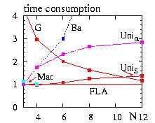 There are several ways to simulate this probability. The fastest is to use the
Fast Linear Algorithm [Loison2004,Loison2004b]. However for almost
similar speed we can use the method that I called the Sinus-Uniform method.
It consists to produce a random number following a probability
sin(x).dx (i.e. cos−1(ran)) and use a rejection method.
This procedure is until 4 times faster than the "standard"
procedure of using N Normal random
numbers and scale them by the the norm of their sum. This property holds
if N < 11. For N ≥ 11 the standard procedure is faster.
Fore more details about the methods and their implementations see
[Loison2004b].
There are several ways to simulate this probability. The fastest is to use the
Fast Linear Algorithm [Loison2004,Loison2004b]. However for almost
similar speed we can use the method that I called the Sinus-Uniform method.
It consists to produce a random number following a probability
sin(x).dx (i.e. cos−1(ran)) and use a rejection method.
This procedure is until 4 times faster than the "standard"
procedure of using N Normal random
numbers and scale them by the the norm of their sum. This property holds
if N < 11. For N ≥ 11 the standard procedure is faster.
Fore more details about the methods and their implementations see
[Loison2004b].
After an instance of the class is created you can use these functions:
| void setParameter(int N) |
|
N is the dimension of the space |
| vector<double> ran( ) |
|
return a vector coordinate of n elements |
| vector<vector<double> > ranVector( ) |
|
return a matrix of L vectors coordinate of n elements each |
Example of program:
// Example Sphere.cpp
// Create L points (4 coordinates) on a sphere
// of 4 dimensions and of radius unity
// check correlations between coordinate =0
// check histogram

#include "LOPOR.hpp"
using namespace LOPOR;

int main( )
{
    try
    {
        // create instance
        Sphere sphere;
        sphere.setParameter(4);

        // results
        std::vector<std::vector<double> > matrix_res;

        // matrix_res={ {a0,b0,c0,d0}, {a1,b1,c1,d1}, …, {aL,bL,cL,dL} }
        matrix_res=sphere.ranVector(100000);

        // matrix_res={ {a0,a1,a2…,aL} , {b0,b1,b2,…,bL} ,…}
        matrix_res=matrix_transposed(matrix_res);

        // check correlation
        print("correlations: exact=0");
        print("correlations x0.x1=",
                vec_mean(vec_multiply( matrix_res[0],matrix_res[1])));
        print("correlations x0.x2=",
                vec_mean(vec_multiply( matrix_res[0],matrix_res[2])));
        print("correlations x0.x3=",
                vec_mean(vec_multiply( matrix_res[0],matrix_res[3])));
        print("correlations x1.x2=",
                vec_mean(vec_multiply( matrix_res[1],matrix_res[2])));
        print("correlations x1.x3=",
                vec_mean(vec_multiply( matrix_res[1],matrix_res[3])));
        print("correlations x2.x3=",
                vec_mean(vec_multiply( matrix_res[2],matrix_res[3])));

        // Construct histogram on [-1:1] with 100 bins with normalization
        // and print in files
        vec_histogram_print("Sphere0.res",matrix_res[0],-1,1,100);
        vec_histogram_print("Sphere1.res",matrix_res[1],-1,1,100);
        vec_histogram_print("Sphere2.res",matrix_res[2],-1,1,100);
        vec_histogram_print("Sphere3.res",matrix_res[3],-1,1,100);
    }
    catch (const Error& error) { error.information( ); }
    return 0;
The output is:
correlations: exact=0
correlations x0.x1= -0.000451172
correlations x0.x2= 0.0010871
correlations x0.x3= -0.000395938
correlations x1.x2= 0.00144457
correlations x1.x3= -0.00150719
correlations x2.x3= 0.000127702
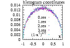
You can plot the column 3 as function of the column 2 of the files
"Sphere0.res", "Sphere1.res", "Sphere2.res", and "Sphere3.res", and
the exact result (with a coefficient to fit the data)
0.013 (1.-x2)½
to check the results.
The class Ball.hpp is
not based on the Distribution
class.
We want to generate points in a ball in N dimensions. The radius of the ball
is 1.
The probability density function is:
f(θ) = dθ0
.sin(θ1).dθ1
.sin2(θ2).dθ2
.sin3(θ3).dθ3
…
.sinN−2(θN−2).dθN−2
.rM−1.dr
with θ is a vector
θ={θ0,θ1,…θN−2}
of N−1 elements.
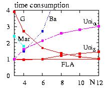 There are several ways to simulate this probability. The fastest is to use the
Fast Linear Algorithm [Loison2004,Loison2004b]. However for almost
similar speed we can use the method that I called the Sinus-Uniform method.
It consists to produce a random number following a probability
sin(x).dx (i.e. cos−1(ran)) and use a rejection method.
This procedure is until 4 times faster than the "standard"
procedure of using N Normal random
numbers and scale them by the the norm of their sum. This property holds
if N < 8. For N ≥ 8 the standard procedure is faster.
Fore more details about the methods and their implementations see
[Loison2004b].
There are several ways to simulate this probability. The fastest is to use the
Fast Linear Algorithm [Loison2004,Loison2004b]. However for almost
similar speed we can use the method that I called the Sinus-Uniform method.
It consists to produce a random number following a probability
sin(x).dx (i.e. cos−1(ran)) and use a rejection method.
This procedure is until 4 times faster than the "standard"
procedure of using N Normal random
numbers and scale them by the the norm of their sum. This property holds
if N < 8. For N ≥ 8 the standard procedure is faster.
Fore more details about the methods and their implementations see
[Loison2004b].
After an instance of the class is created you can use these functions:
| void setParameter(int N) |
|
N is the dimension of the space |
| vector<double> ran( ) |
|
return a vector coordinate of n elements |
| vector<vector<double> > ranVector( ) |
|
return a matrix of L vectors coordinate of n elements each |
Example of program:
// Example Ball.cpp
// Create L points (4 coordinates) on a ball
// of 4 dimensions and of radius unity
// check correlations between coordinate =0

#include "LOPOR.hpp"
using namespace LOPOR;

int main( )
{
    try
    {
        // create instance
        Ball ball;
        ball.setParameter(4);

        // results
        std::vector<std::vector<double> > matrix_res;

        // matrix_res={ {a0,b0,…}, {a1,b1,…}, …, {aL,bL,…} }
        matrix_res=ball.ranVector(100000);

        // matrix_res={ {a0,a1,a2…,aL} , {b0,b1,b2,…,bL} ,…}
        matrix_res=matrix_transposed(matrix_res);

        // check correlation
        print("correlations: exact=0");
        print("correlations x0.x1=",
                vec_mean(vec_multiply( matrix_res[0],matrix_res[1])));
        print("correlations x0.x2=",
                vec_mean(vec_multiply( matrix_res[0],matrix_res[2])));
        print("correlations x0.x3=",
                vec_mean(vec_multiply( matrix_res[0],matrix_res[3])));
        print("correlations x1.x2=",
                vec_mean(vec_multiply( matrix_res[1],matrix_res[2])));
        print("correlations x1.x3=",
                vec_mean(vec_multiply( matrix_res[1],matrix_res[3])));
        print("correlations x2.x3=",
                vec_mean(vec_multiply( matrix_res[2],matrix_res[3])));
    }
    catch (const Error& error) { error.information( ); }
    return 0;
The output is:
correlations: exact=0
correlations x0.x1= 0.000397152
correlations x0.x2= -7.3353e-05
correlations x0.x3= 0.000742098
correlations x1.x2= 3.76237e-05
correlations x1.x3= -0.000492953
correlations x2.x3= 0.000487361
The quasi random number methods, for example Sobol, Faure or Halton methods,
are a tentative to fill the configuration space more uniformly
than a uniform random number. In a sense we want to have the benefit
of the Latin hypercubic method [Loison2004]
with less correlation problems. However the method still
produce some correlations and you should be careful when using it.
For the finance it is usually not problematic if you are not searching a
result with an accuracy less than 0.01%. Moreover the methods
does not increases the performance compared to an uniform random
number generator for high dimensions. For more information you could
refer to Numerical Recipes,
[Jackel2002] and
[London2005].
The static functions available within the class "Sobol.hpp" are:
| static vector<double> Sobol::ran(int n) |
|
return a vector of n quasi uniform random numbers between 0 and 1. |
| static vector<vector<double> > Sobol::ranVector(int n, int L) |
|
return a matrix of L vectors of n quasi uniform random numbers between 0 and 1. |
An example of program:
// Example Sobol.cpp

#include "LOPOR.hpp"
using namespace LOPOR;

int main( )
{
    try
    {
        for(int i=0; i<10; ++i)
        {
            std::vector<double> res1=Sobol::ran(2);
            print(res1[0],res1[1]);
        }
    }
    catch (const Error& error) { error.information( ); }
    return 0;
}
And the output is:
0.5 0.5
0.25 0.75
0.75 0.25
0.375 0.625
0.875 0.125
0.125 0.375
0.625 0.875
0.3125 0.3125
0.8125 0.8125
0.0625 0.5625
As you can see, the "random" numbers are not random at all and display
definite correlations. However if we plot
500 points and compare it with the plot with an uniform random number,
we observe that the space is more uniformly covert with the Sobol
sequence.
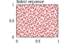
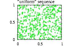
The class PolynomeMulti_fc.hpp is not based on the Distribution class.
The PolynomeMulti_fc class defined the function
f(x) = a0 + a1x0 + a2x02
+ a3x1 + a4x12
+ a5 x0x1 + …
No random number generator is provided and the function is mainly used
for the fit. The functions accessible are:
|
void
setParameter(vector<int> degree) |
|
degree={2,1} for example. Gives the order
the polynome for each variable. |
|
string information( ) |
|
return information about the order of the polynomes |
|
double density(vector<double> x) |
|
return f(x) |
|
vector<double> fit(vector<vector<double>> dataX, vector<double> dataY, vector<double> σ) |
|
Fit and update the parameters. To have information of the order of parameters,
call the information( ) function. |
Example:
// Example PolynomeMulti.cpp
// Create polynome in 2 dimensions and fit with data

#include "LOPOR.hpp"
using namespace LOPOR;

int main( )
{
    try
    {
        // create data
        std::vector<std::vector<double> > dataX;
        std::vector<double> dataY;

        for(int i=0; i<100; ++i)
        {
            double x1=(i/10.);
            double x2=(i/10.);
            dataX.push_back(c2v(x1,x2));
            dataY.push_back(22.+33.*x1+3.7*x1*x1+2.5*x1*x2+0.1*x1*x1*x2+12*x2);
        }

        // create instance
        PolynomeMulti_fc polynome;

        // define f(x1,x2)= a + b.x1 + c.x1^2 + d.x1x2 + e.x1^2.x2 + f.x2
        polynome.setParameter(c2v<int>(2,1));
        print("before fit:"+polynome.information());

        // fit
        std::vector<double> res=polynome.fit(dataX,dataY);
        print("after  fit:"+polynome.information());


        // print results res={Parameters, sigma, chi^2}
        print("\nResult with error:");
        for(int k=0; k<(res.size()-1)/2; ++k)
            print( res[k], "+/-", res[k+(res.size()-1)/2]);
        print("chi^2=",res[res.size()-1]);

        // print results : we should have fit_result=dataY
        std::vector<double> fit_result, X1, X2;
        for(int i=0; i<100; ++i)
        {
            fit_result.push_back(polynome.density(dataX[i]));
            X1.push_back(dataX[i][0]);
            X2.push_back(dataX[i][1]);
        }
        vec_print("res.res",X1,X2,dataY,fit_result);

    }
    catch (const Error& error) { error.information( ); }
    return 0;
}
And the output is:
before fit:LOPOR::PolynomeMulti_fc( 1 +1.x[0] +1.x[0]^2 +1.x[1] +1.x[0].x[1] +1.x[0]^2.x[1] )
power x[i][j]  + Parameters[i]
j=0, j=1,  Parameters=
0     0        1
1     0        1
2     0        1
0     1        1
1     1        1
2     1        1

after  fit:LOPOR::PolynomeMulti_fc( 22 +22.5.x[0] +3.1.x[0]^2 +22.5.x[1] +3.1.x[0].x[1] +0.1.x[0]^2.x[1] )
power x[i][j]  + Parameters[i]
j=0, j=1,  Parameters=
0     0        22
1     0        22.5
2     0        3.1
0     1        22.5
1     1        3.1
2     1        0.1


Result with error:
22 +/- 0.385457
22.5 +/- 0.169443
3.1 +/- 0.0398854
22.5 +/- 0.169443
3.1 +/- 0.0398854
0.1 +/- 0.00529521
chi^2= 5.19251e-23
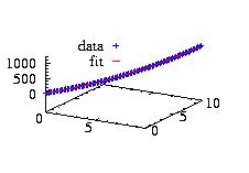
Plot of the file "res.res" using the columns 2 and 3
as x0 and x1, the 4th
for the data, and the 5th for the fit.
The class Fit provides several possible fits as static functions. A problem of fitting can be divided in several types.
You have a serie of results, for example the losses of your bank like
(scale 1000$)
{1,2.3,1.1,0.4,100.2,80.7,…}, you know that it comes from a
distribution and you would like to calculate its parameters.
There are several ways: method of moments, method of maximum
likelihood, least squares fitting.
Remark: If you have the x and the cumulative F(x), you should go to the
section Cumulative 2
The method of moments uses the moments of the distribution (average, variance,…) to calculate the parameters of the distribution. We have defined a static function in the class Fit:
| vector <double> static Fit::Moments(Distribution* dist,vector <double> vecX) |
|
*dist is the address of the
distribution, |
// Example Fit_Moments.cpp (download)
#include "LOPOR.hpp"
using namespace LOPOR;

int main( )
{
    try
    {
        Logistic dist;            //define the distribution

          // create data
        dist.setParameter(0,0.2); // define parameters
        std::vector <double>  vecX(dist.ranVector(50)); //create data
        print("data   from: ",dist.information( ));   // display information

        dist.setParameter(1,0.5); // change the parameters
        print("before fit : ",dist.information( ));   // display information

          // fit
        std::vector <double>  results=Fit::Moments(&dist,vecX);

          // display result and information
        print("after  fit : ",dist.information( ));
        vec_print(results,"results of the fit");

          // compare data with the cumulative
        vecX=vec_sort(vecX);      // sort to use vec_cumulative
        vec_print("data_cumulative.res",vecX,vec_cumulative(vecX));
        vec_print("dist_cumulative.res",vecX,dist.cumulativeVector(vecX));
    }
    catch (const LOPOR::Error& error) { error.information( ); }
    return 0;
}
The output of the program is:
data   from:  LOPOR::Logistic(0,0.2)
before fit :  LOPOR::Logistic(1,0.5)
after  fit :  LOPOR::Logistic(0.00121365,0.180511)
#   i=      results of the fit
     0     0.00121365
     1       0.180511
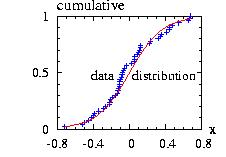 And you can print the files "data_cumulative.res" and "dist_cumulative.res"
using the second in abscissa and the third in ordinate to obtain the
figure.
With gnuplot we have: the command
And you can print the files "data_cumulative.res" and "dist_cumulative.res"
using the second in abscissa and the third in ordinate to obtain the
figure.
With gnuplot we have: the command
p 'data_cumulative.res' u 2:3, 'dist_cumulative.res' u 2:3 w l
We can see that the method of moment does not give bad
results.
The maximum Likelihood Estimator (MLE) can be seen as a generalization of the method of moments and for some distributions results are similar. We have defined a static function in the class Fit:
| vector <double> static Fit::MLE(Distribution* dist,vector <double> vecX) |
|
*dist is the address of the
distribution, |
// Example Fit_MLE.cpp (download)
#include "LOPOR.hpp"
using namespace LOPOR;

int main( )
{
    try
    {
        Logistic dist;            //define the distribution

          // create data
        dist.setParameter(0,0.2); // define parameters
        std::vector <double>  vecX(dist.ranVector(50)); //create data
        print("data   from: ",dist.information( ));   // display information

        dist.setParameter(1,0.5); // change the parameters
        print("before fit : ",dist.information( ));   // display information

          // fit
        std::vector <double>  results=Fit::MLE(&dist,vecX);

          // display result and information
        print("after  fit : ",dist.information( ));
        vec_print(results,"results of the fit");

          // compare data with the cumulative
        vecX=vec_sort(vecX);      // sort to use vec_cumulative
        vec_print("data_cumulative.res",vecX,vec_cumulative(vecX));
        vec_print("dist_cumulative.res",vecX,dist.cumulativeVector(vecX));
    }
    catch (const LOPOR::Error& error) { error.information( ); }
    return 0;
}
The output of the program is:
data   from:  LOPOR::Logistic(0,0.2)
before fit :  LOPOR::Logistic(1,0.5)
after  fit :  LOPOR::Logistic(-0.0138991,0.186068)
#   i=      results of the fit
     0     -0.0138991
     1       0.186068
 And you can print the files "data_cumulative.res" and "dist_cumulative.res"
using the second in abscissa and the third in ordinate to obtain the
figure.
With gnuplot we have: the command
And you can print the files "data_cumulative.res" and "dist_cumulative.res"
using the second in abscissa and the third in ordinate to obtain the
figure.
With gnuplot we have: the command
p 'data_cumulative.res' u 2:3, 'dist_cumulative.res' u 2:3 w l
The Maximum Likelihood Estimator gives almost the same results as the
method of Moments.
The method uses a function based on derivatives of the cumulative to minimize the distance between the data and the cumulative. In the great majority of the case we have the vecX alone which is a random sampling of one distribution. In this case the cumulative from the data is constructed using vec_cumulative. This case is explained in this section. However for some cases we could have the vecY, the value of the cumulative. This case is explained in the section Cumulative2. We have defined a static function in the class Fit:
| vector <double> static Fit::LeastSquares_LM_cum(Distribution* dist,vector <double> vecX) |
|
*dist is the address of the
distribution, |
It is absolutely not sure that the fit would converge.
Usually it
would not if the initial guess of the parameters (the actual in the
distribution) is too far away of a solution. For example, if we try to run the last program
changing only the method from MLE to
LeastSquares_LM_cum, it will produce an error. The solution consists
to call the function Fit::Moments and/or
Fit::MLE before calling the function
Fit::LeastSquares_LM_cum.
Another problem is that it is sometimes difficult to calculate the derivative
of the cumulative and therefore the method is not accessible for all distributions.
For these distributions, and if you are not satisfied with the method of
Moments and the Maximum Likelihood Estimator
(MLE), you can use the vec_histogramY
and vec_histogramX functions
to produce some data (x,f(x)) and use the
LeastSquares_LM_den to fit the
density.
To keep some parameters constant you should define them constant in the
distribution using fit_keep.
Example of use of Fit::LeastSquares_LM_cum:
// Example Fit_LeastSquares_LM_cum1.cpp (download)
#include "LOPOR.hpp"
using namespace LOPOR;

int main( )
{
    try
    {
        Logistic dist;            //define the distribution

          // create data
        dist.setParameter(0,0.2); // define parameters
        std::vector <double>  vecX(dist.ranVector(50)); //create data
        print("data   from  :",dist.information( ));   // display information

        dist.setParameter(1,0.5); // change the parameters
        print("before fit   :",dist.information( ));   // display information

          // fit
          // Fit Moments
        try{ Fit::Moments(&dist,vecX);}
        catch (const LOPOR::Error& error) { error.information( ); }
        print("after Moments:",dist.information( ));

          // Fit MLE
        try{ Fit::MLE(&dist,vecX);}
        catch (const LOPOR::Error& error) { error.information( ); }
        print("after MLE    :",dist.information( ));

          // Fit LeastSquares_LM_cum + keep the first parameter const
        dist.fit_keep =c2v <int> (0);
        Fit::LeastSquares_LM_cum(&dist,vecX);
        print("after fit+keep",dist.information( ));

          // fit LeastSquares_LM_cum, no parameter kept cst
        dist.fit_keep.clear( );
        std::vector <double>  results=Fit::LeastSquares_LM_cum(&dist,vecX);

          // display result and information
        print("after  fit   :",dist.information( ));
        vec_print(results,"results of the fit");

          // compare data with the cumulative
        vecX=vec_sort(vecX);      // sort to use vec_cumulative
        vec_print("data_cumulative.res",vecX,vec_cumulative(vecX));
        vec_print("dist_cumulative.res",vecX,dist.cumulativeVector(vecX));
    }
    catch (const LOPOR::Error& error) { error.information( ); }
    return 0;
}
The output of the program is:
data   from  : LOPOR::Logistic(0,0.2)
before fit   : LOPOR::Logistic(1,0.5)
after Moments: LOPOR::Logistic(0.00121365,0.180511)
after MLE    : LOPOR::Logistic(-0.0138991,0.186068)
after fit+keep LOPOR::Logistic(-0.0138991,0.193794)
after  fit   : LOPOR::Logistic(-0.0320585,0.188705)
#   i=      results of the fit
     0     -0.0320585
     1       0.188705
     2      0.0214529
     3      0.0297845
which means parameter1=-0.0320585±0.0214529 and
parameter2=0.188705±0.0297845;
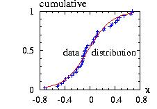 You can print the files "data_cumulative.res" and "dist_cumulative.res"
using the second in abscissa and the third in ordinate to obtain the
figure.
With gnuplot we have: the command
You can print the files "data_cumulative.res" and "dist_cumulative.res"
using the second in abscissa and the third in ordinate to obtain the
figure.
With gnuplot we have: the command
p 'data_cumulative.res' u 2:3, 'dist_cumulative.res' u 2:3 w l
The Maximum Likelihood Estimator gives almost similar
result as the
method of Moments
and the Maximum Likelihood Estimator (MLE).
The second example is a little bit more complicated.
// Example LeastSquares_LM_cum2.cpp  download
#include "LOPOR.hpp"
using namespace LOPOR;

int main( )
{
    try
    {
        std::vector <double>  vecX, result;

        // DEFINE DISTRIBUTIONS
        // you can see the density for the following distributions  below
        Geometric   geo  ;
        Binomial    bin  ;
        Translate   trans;
        Interval    inter;
        Sum         sum  ;

        // PREPARE THE DATA
        geo.setParameter(0.4);
        bin.setParameter(10,0.5);
            // bin is translated by -2
        trans.setParameter(&bin,-2);
            // last parameter=border=2 : keep only of
            // trans=bin_translated  the data from [4,oo[
            // with border=2 the max=10 is ignored
        inter.setParameter(&trans,4,10,2);
            //sum
        sum.setParameter(c2v < Distribution * > (&geo,&inter));
            // random sampling : 50 data
        vecX=sum.ranVector(50);
        print("data   from   :",sum.information( ));   // display information

        // CONSTANT PARAMETER FOR THE FIT
        // -The first parameter for bin : n=10 is always kept constant
        //   with LeastSquares_LM_cum, no need to repeat it
        // -The translation -2 should be kept constant for the fit
        //   It is the last parameter for trans (number 2):
        //   trans.get_Parameters( )={10,0.5,-2}
        //   the two first come from the distribution bin.
        // -The three last parameters for inter (4,10,2) are always kept constant
        //   with LeastSquares_LM_cum, no need to repeat it
        trans.fit_keep=c2v <int> (trans.get_Parameters( ).size( )-1);

        // CHANGE PARAMETERS OF THE DISTRIBUTIONS
        //   the sum will be automatically updated
        bin.setParameter(10,0.6);
        geo.setParameter(0.6);
        print("Before fit    :",sum.information( ));   // display information

        // FIT LeastSquares_LM_cum
        result=Fit::LeastSquares_LM_cum(&sum,vecX);

        // DISPLAY RESULT AND INFORMATION
        print("After  fit    :",sum.information( ));   // display information
        vec_print(result,"Sum Parameters");

        // COMPARE DATA WITH THE CUMULATIVE
        vecX=vec_sort(vecX);      // sort to use vec_cumulative
        vec_print("data.res",vecX,vec_cumulative(vecX));
        vec_print("sum.res" ,vecX,sum.cumulativeVector(vecX));

    }
    catch (const LOPOR::Error">Error& error) { error.information( ); }
    return 0;
}
The output of the program is:
data   from   : LOPOR::Sum::Sum({D}): D.size( )=2
LOPOR::Geometric(0.4)
LOPOR::Interval(LOPOR::Binomial(10,0.5)- > Translated(x- > x+X0=x+-2),[4,+oo])

Before fit    : LOPOR::Sum::Sum({D}): D.size( )=2
LOPOR::Geometric(0.6)
LOPOR::Interval(LOPOR::Binomial(10,0.6)- > Translated(x- > x+X0=x+-2),[4,+oo])

After  fit    : LOPOR::Sum::Sum({D}): D.size( )=2
LOPOR::Geometric(0.398805)
LOPOR::Interval(LOPOR::Binomial(10,0.475149)- > Translated(x- > x+X0=x+-2),[4,+oo])

#   i=      Sum Parameters       (Comments:added: not output)
     0       0.398805                   pgeo                  Parameters
     1             10                        nbin
     2       0.475149                   pbin
     3             -2                         x0-trans
     4              4                         Ainter
     5             10                        Binter
     6              2                         borderinter   ______________________
     7      0.0474359                  error_pgeo                  Errors
     8              0                         nbin kept cst
     9       0.276627                  error_pbin
    10              0                         x0-trans kept cst
    11              0                         Ainter kept cst
    12              0                         Binter kept cst
    13              0                         borderinter kept cst
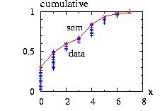
You can print the files "data.res" and "sum.res"
using the second in abscissa and the third in ordinate to obtain the
figure.
With gnuplot we have: the command
p 'data.res' u 2:3 ,'sum.res' u 2:3 w lp
For these discrete distributions the top of the point of "data"
should cross the line "sum" if it was in complete accordance.
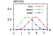
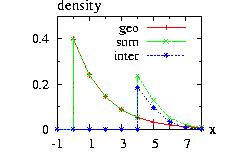
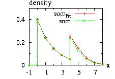
You can fit the cumulative with any function, and not only the Least Square Method, using the Minimum function and in particular the Annealing method. See Example Annealing.cpp. In this example the Least square Method is implemented. You can easily change the function.
You have at least two vectors vecX and vecY corresponding to x and the cumulative F(x). You can also have the error on F(x). If you have only a random sampling of data, vecX, please go Cumulative1. We have defined a static function in the class Fit:
| vector <double> static Fit::LeastSquares_LM_cum(Distribution* dist,vector <double> vecX,vector<double > vecY,vector<double > ErrorY=vector_NULL<double > ( )) |
|
*dist is the address of the
distribution, |
It is absolutely not sure that the fit would converge and usually it
would not if the initial guess of the parameters (the actual in the
distribution) is too far away of a solution.
To keep some parameters constant you should define them constant in the
distribution using fit_keep.
Example of use of Fit::LeastSquares_LM_cum:
// Example LeastSquares_LM_cum3.cpp  download
#include "LOPOR.hpp"
using namespace LOPOR;

int main( )
{
    try
    {
        std::vector <double>  vecX,vecY,vecRan,results;

        Logistic dist;            //define the distribution
        dist.setParameter(0,0.2); // define parameters
        print("data   from   :",dist.information( ));   // display information

          // create data
        vecX=vec_create(51,-1.,0.04); //create data X={-1,-0.96,…,+1)
        vecY=dist.cumulativeVector(vecX); //create data Y
          //random vector between 0.9 to 1.1
        vecRan=vec_add(vec_multiply(Random::ranVector(51),0.2),0.9);
          // put some random in vecY= vecY *r with r vary randomly from 0.9 to 1.1
        vecY=vec_multiply(vecY,vecRan);


        dist.setParameter(0,0.5); // change the parameters
        print("before fit    :",dist.information( ));   // display information

          // fit LeastSquares_LM_cum,
          // no error is given: give a null vector
          // keep the first parameter const
        dist.fit_keep=c2v(0);
        results=Fit::LeastSquares_LM_cum(&dist,vecX,vecY);
        print("after fit+keep:",dist.information( ));
        vec_print(results,"results of the fit+keep");

          // fit LeastSquares_LM_cum, no error, no keep
        dist.fit_keep.clear( );
        results=Fit::LeastSquares_LM_cum(&dist,vecX,vecY);
        print("after  fit    :",dist.information( ));
        vec_print(results,"results of the fit");

          // compare data with the cumulative
        vec_print("data.res",vecX,vecY);
        vec_print("dist_cumulative.res",vecX,dist.cumulativeVector(vecX));
    }
    catch (const LOPOR::Error& error) { error.information( ); }
    return 0;
}
The output of the program is:
data   from   : LOPOR::Logistic(0,0.2)
before fit    : LOPOR::Logistic(0,0.5)
after fit+keep: LOPOR::Logistic(0,0.194)
#   i=      results of the fit+keep
     0              0
     1          0.194
     2              0
     3      0.0362468
after  fit    : LOPOR::Logistic(-0.000128358,0.194002)
#   i=      results of the fit
     0   -0.000128358
     1       0.194002
     2      0.0465678
     3      0.0362471
For the first case with the first parameter kept constant the results are
parameter1=0±0 and parameter2=0.194±0.0362468.
For the second case with no constant parameter we obtain
parameter1=-0.000128358±0.0465678 and
parameter2=0.194002±0.0362471.
You can fit the cumulative with any function, and not only the Least Square Method, using the Minimum function and in particular the Annealing method. See Example Annealing.cpp. In this example the Least square Method is implemented. You can easily change the function.
You have now a serie of results (x,y,error) for various x and you want to fit the data by a distribution. You could have made this data using the vec_histogramX or the vec_histogramY from data which is a random sampling for one distribution:
// vec is a vector, random sampling of a distribution
std::vector < double< vecX=vec_middle(vec_histogramX(vec,-0.5,+0.5,10));
std::vector < double< vecY=vec_histogramY(vec,-0.5,+0.5,10);
Or you got it from a source and you cannot get the initial data,
or for one reason or another you have a histogram, i.e. a vector
vecX, a vector vecY, and sometimes you have access to the error of Y
under the form ErrorY.
You want fit these data to the density of a distribution.
You want to fit your data by a polynome(x)=a0+a1x+a2x2+a3x3+… and therefore estimate the parameters ai. The static function Fit::Polynome has this syntax:
| vector <double> static Fit::Polynome(int degree,vector <double> vecX, vector<double > vecX, vector <double> ErrorY=vec_NULL<int > ) |
|
degree is the degree the polynome: a0,…,adegree |
Example:
// Example Polynome.cpp (download)
#include "LOPOR.hpp"
using namespace LOPOR;

int main( )
{
    try
    {
          // data
        std::vector <double>  vecX  =c2v<double > (0  ,1 ,2  ,3  ,4  ,5  ,6  );
        std::vector <double>  vecY  =c2v<double > (0.1,1.,1.9,3.2,4.1,5.0,6.2);
        std::vector <double>  ErrorY=c2v<double > (0.1,0.05,0.2,0.1,0.1,0.2,0.05);

          // Fit
        int degree=1;
        std::vector <double>  resPara=Fit::Polynome(degree,vecX,vecY);

          // Display results
        vec_print(resPara,"results");

          // create the vector results to compare to data
          // f(x) = a0 + x^1 * a1
        std::vector <double>  resY(degree);
        for(int i=0; i < =degree; ++i)
            resY=vec_add( resY , vec_multiply( vec_power(vecX,i), resPara[i] ) );
        vec_print("results.res",vecX,resY);
        vec_print("data.res"  ,vecX,vecY,ErrorY);
    }
    catch (const LOPOR::Error& error) { error.information( ); }
    return 0;
}
The output of the program is:
#   i=      results
     0    0.000666263
     1        1.03176
     2      0.0499546
     3      0.0126179
Which means that a0=0.000666263 ± 0.0499546 and
a1=1.03176 ± 0.0126179
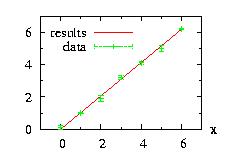
You can print the files "data.res" and "results.res"
using the second in abscissa and the third in ordinate to obtain the
figure.
With gnuplot we have: the command
p 'results.res' u 2:3 w l,'data.res' u 2:3:4 w e
You want to fit your data by an exponential(x)=ea0+a1x+a2x2+a3x3+… and therefore estimate the parameters ai. The static function Fit::Exponential has this syntax:
| vector <double> static Fit::Exponential(int degree,vector <double> vecX, vector<double > vecX, vector <double> ErrorY=vec_NULL<double > ) |
|
degree is the degree the polynome: a0,…,adegree |
Example:
// Example Fit_Exponential.cpp (download)
#include "LOPOR.hpp"
using namespace LOPOR;

int main( )
{
    try
    {
          // data
        std::vector <double>  vecX  =c2v<double > (0  ,1 ,2  ,3  ,4  ,5  ,6  );
        std::vector <double>  vecY  =c2v<double > (0.1,1.,1.9,3.2,4.1,5.0,6.2);
        std::vector <double>  ErrorY=c2v<double > (0.05,0.1,0.2,0.15,0.2,0.2,0.3);

          // Fit
        int degree=2;
        std::vector <double>  resPara=Fit::Exponential(degree,vecX,vecY,ErrorY);

          // Display results
        vec_print(resPara,"results");

          // create the vector results to compare to data
          // f(x) = exp(a0 + x^1 * a1)
        std::vector <double>  resY(degree);
        for(int i=0; i < =degree; ++i)
            resY=vec_add( resY , vec_multiply( vec_power(vecX,i), resPara[i] ) );
        resY=vec_exp(resY);
        vec_print("results.res",vecX,resY);
        vec_print("data.res"  ,vecX,vecY,ErrorY);
    }
    catch (const LOPOR::Error& error) { error.information( ); }
    return 0;
}
The output of the program is:
#   i=      results
     0      -0.733996
     1         0.8012
     2     -0.0640663
     3      0.0212576
     4     0.00609736
     5    9.80883e-05
Which means that a0=-0.733996 ± 0.0212576,
a1=0.8012 ± 0.00609736 and a2=-0.0640663 ± 9.80883e-05.
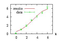
You can print the files "data.res" and "results.res"
using the second in abscissa and the third in ordinate to obtain the
figure.
With gnuplot we have: the command
p 'results.res' u 2:3 w l,'data.res' u 2:3:4 w e
You can apply this method if the function to fit is of the form:
f(x) = a0 g0(x) + a1 g1(x) + …
and gi(x) could be any function. The class LeastSquares_Linear_den
function fit the ai if you give a vector X and a vector Y.
To use this function, the function
fit_den_linear() must be defined for the
distribution.
We have defined a static function in the class Fit:
| vector <double> static Fit::LeastSquares_Linear_den(Distribution* dist,vector <double> vecX, vector <double> vecY,vector<double > ErrorY=vec_NULL<double > ) |
|
*dist is the address of the
distribution, |
Remark: you cannot keep some parameters constant.
Example of use of Fit::LeastSquares_Linear_den:
// Example LeastSquares_Linear_den1.cpp
#include "LOPOR.hpp"

using namespace LOPOR;
int main()
{
    try
    {
        std::vector<double> vecX,vecY,vecRan,results;

        Polynome_fc dist;            //define the distribution
        dist.setParameters(c2v(1.,1.5,0.5)); // define parameters
        print("data   from   :",dist.information());   // display information

          // create data
        vecX=vec_create(51,-1.,0.04); //create data X={-1,-0.96,…,+1)
        vecY=dist.densityVector(vecX); //create data Y
          //random vector between 0.9 to 1.1
        vecRan=vec_add(vec_multiply(Random::ranVector(51),0.2),0.9);
          // put some random in vecY= vecY *r with r vary randomly from 0.9 to 1.1
        vecY=vec_multiply(vecY,vecRan);


        dist.setParameters(c2v(2.,2.5,2.5)); // change the parameters
        print("before fit    :",dist.information());   // display information

          // fit LeastSquares_Linear_den, no error,
        results=Fit::LeastSquares_Linear_den(&dist,vecX,vecY);
        print("after  fit    :",dist.information());
        vec_print(vec_remove(results,3,6),vec_remove(results,0,3),"results  +-");

          // compare data with the density
        vec_print("data.res",vecX,vecY);
        vec_print("dist_density.res",vecX,dist.densityVector(vecX));
    }
    catch (const LOPOR::Error& error) { error.information(); }
    return 0;
}
The output of the program is:
data   from   : LOPOR::Polynome_fc( 1*x^0 + 1.5*x^1 + 0.5 x^2 )
before fit    : LOPOR::Polynome_fc( 2*x^0 + 2.5*x^1 + 2.5 x^2 )
after  fit    : LOPOR::Polynome_fc( 0.989684*x^0 + 1.52849*x^1 + 0.576792 x^2 )
#   i=      results  +-
     0   0.989684   0.044146
     1    1.52849  0.0565611
     2   0.576792   0.204182
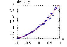
you can print the files "data.res" and "dist_density.res"
using the second in abscissa and the third in ordinate to obtain the
figure.
With gnuplot we have: the command
p 'data.res' u 2:3, 'dist_density.res' u 2:3 w l
The method uses a function based on derivatives of the density
to minimize the distance between the data and the density.
We have defined a static function in the class Fit:
| vector <double> static Fit::LeastSquares_LM_den(Distribution* dist,vector <double> vecX, vector <double> vecY,vector<double > ErrorY=vec_NULL<double > ) |
|
*dist is the address of the
distribution, |
It is absolutely not sure that the fit would converge and usually it
would not if the initial guess of the parameters (the actual in the
distribution) is too far away of a solution.
Example of use of Fit::LeastSquares_LM_den:
// Example LeastSquares_LM_den1.cpp download
#include "LOPOR.hpp"
using namespace LOPOR;

int main( )
{
    try
    {
        std::vector <double>  vecX,vecY,vecRan,results;

        Logistic dist;            //define the distribution
        dist.setParameter(0,0.2); // define parameters
        print("data   from   :",dist.information( ));   // display information

          // create data
        vecX=vec_create(51,-1.,0.04); //create data X={-1,-0.96,…,+1)
        vecY=dist.densityVector(vecX); //create data Y
          //random vector between 0.9 to 1.1
        vecRan=vec_add(vec_multiply(Random::ranVector(51),0.2),0.9);
          // put some random in vecY= vecY *r with r vary randomly from 0.9 to 1.1
        vecY=vec_multiply(vecY,vecRan);


        dist.setParameter(0,0.5); // change the parameters
        print("before fit    :",dist.information( ));   // display information

          // fit LeastSquares_LM_den,
          // no error is given: give a null vector
          // keep the first parameter const
        dist.fit_keep=c2v(0);
        results=Fit::LeastSquares_LM_den(&dist,vecX,vecY);
        print("after fit+keep:",dist.information( ));
        vec_print(results,"results of the fit+keep");

          // fit LeastSquares_LM_den, no error, no keep
        dist.fit_keep.clear( );
        results=Fit::LeastSquares_LM_den(&dist,vecX,vecY);
        print("after  fit    :",dist.information( ));
        vec_print(results,"results of the fit");

          // compare data with the density
        vec_print("data.res",vecX,vecY);
        vec_print("dist_density.res",vecX,dist.densityVector(vecX));
    }
    catch (const LOPOR::Error& error) { error.information( ); }
    return 0;
}
The output of the program is:
data   from   : LOPOR::Logistic(0,0.2)
before fit    : LOPOR::Logistic(0,0.5)
after fit+keep: LOPOR::Logistic(0,0.201932)
#   i=      results of the fit+keep
     0              0
     1       0.201932
     2              0
     3     0.00302623
after  fit    : LOPOR::Logistic(-0.00169153,0.201911)
#   i=      results of the fit
     0    -0.00169153
     1       0.201911
     2     0.00988955
     3      0.0030253
For the first case with the first parameter kept constant the results are
parameter1=0±0 and parameter2=0.201932±0.00302623.
For the second case with no constant parameter we obtain
parameter1=-0.00169153±0.00988955 and
parameter2=0.201911±0.0030253.
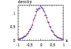
you can print the files "data.res" and "dist_density.res"
using the second in abscissa and the third in ordinate to obtain the
figure.
With gnuplot we have: the command
p 'data.res' u 2:3, 'dist_density.res' u 2:3 w l
You can fit the density with any function, and not only the Least Square Method, using the Minimum function and in particular the Annealing method. See Example Annealing.cpp. In this example the Least square Method is implemented. You can easily change the function.
The χ2 is defined as:
χ2=∑i
[ ni-fi
]2 / fi
i varies from 1 to N, N is the number of histogram (interval or value for discrete distribution),
ni is the number of
observed data for the ith interval or value,
and fi is the frequency that we should observe
if the data comes from the considered distribution.
There are two possible implementations of this quantity following that the distribution
has a double type (continuous distribution): go,
or an integer type (discrete distribution): go .
When you have χ2 (see below), you can calculate
There are two possibilities: You make yourself the histograms (better)
or you let the class do it for you. The first possibility is better because
you have more control on what you are doing. The main point is that the
χ2 is very sensitive to the low density, i.e. the lowest
value of the histogram, and a good control of the histogram is fundamental.
Moreover χ2 is proportional to the number of bins therefore a good choice
of number is also fundamental.
For most situations Scott's Normal approximation for the number of bins will give
a reasonable result:
number of histogram=N=(4*number of data)2/5.
| vector <double> static Fit::Chi_Test(Distribution* dist,vector <double> vecX, vector<double > vecY, int border=3, int a=0) |
|
Return a vector= {χ2,degree of freedom, confidence} |
Or, without creating the histogram, you can send directly the raw data directly to the function and let the function create the histogram:
| vector <double> static Fit::Chi_Test(Distribution* dist,vector <double> data, vector<double > vecY=vec_NULL<double>, int border=3, int a=0) |
|
Return a vector= {χ2,degree of freedom, confidence} |
Example 1:
// Example Chi_Test1.cpp  download
// make yourself the histogram
#include "LOPOR.hpp"
using namespace LOPOR;

int main( )
{
    try
    {
        std::vector <double>  vecX,vecY,vecRan,results;

        Logistic dist;            // define the distribution
        dist.setParameter(20,4);  // define parameters
        print("data   from   :",dist.information( ));   // display information

        vecRan=dist.ranVector(2000);  // random sampling

        // HISTOGRAM:
        // number of interval (4*2000)^(2/5)=36
        // min=-2 and max=42 : statistic of first and last interval not so small
        // type=double : Logistic is a continuous distribution
        // border=3: the interval are: ]-oo,-0,0.78[,[-0.78,0.44[,…,[40.78,+oo[
        vecX=vec_histogramX(vecRan,-2,42,36,"double",3);
        vecY=vec_histogramY(vecRan,-2,42,36,"double",3);

        results=Fit::Chi_Test(&dist,vecX,vecY);
        vec_print(results,"results: Chi^2, degree freedom, confidence");
        vec_print(vecX,vecY,"histogramX, histogramY");
    }
    catch (const LOPOR::Error& error) { error.information( ); }
    return 0;
}
The output of this program is:
data   from   : LOPOR::Logistic(20,4)
#   i=      results: Chi^2, degree freedom, confidence
     0        29.2592
     1             35
     2       0.741119
#   i=      histogramX, histogramY
     0             -2              9
     1      -0.777778              1
     2       0.444444              3
     3        1.66667              7
     4        2.88889             11
     5        4.11111             13
     6        5.33333             10
     7        6.55556             18
     8        7.77778             28
     9              9             40
    10        10.2222             56
    11        11.4444             69
    12        12.6667             88
    13        13.8889            102
    14        15.1111            134
    15        16.3333            143
    16        17.5556            161
    17        18.7778            155
    18             20            156
    19        21.2222            134
    20        22.4444            133
    21        23.6667             96
    22        24.8889            102
    23        26.1111             78
    24        27.3333             54
    25        28.5556             44
    26        29.7778             47
    27             31             27
    28        32.2222             20
    29        33.4444             17
    30        34.6667             12
    31        35.8889              7
    32        37.1111              7
    33        38.3333              8
    34        39.5556              1
    35        40.7778              9
    36             42
Example 2:
// Example Chi_Test2.cpp download
// From raw data
#include "LOPOR.hpp"
using namespace LOPOR;

int main( )
{
    try
    {
        std::vector <double>  vecX,vecY,vecRan,results;

        Logistic dist;            // define the distribution
        dist.setParameter(20,4);  // define parameters
        print("data   from   :",dist.information( ));   // display information

        vecRan=dist.ranVector(2000);  // random sampling

        vecX=vecRan;
        vecY=vec_NULL <double> ( );

        results=Fit::Chi_Test(&dist,vecX,vecY);
        vec_print(results,"results: Chi^2, degree freedom, confidence");
        vec_print(vecX,vecY,"histogramX, histogramY");
    }
    catch (const LOPOR::Error& error) { error.information( ); }
    return 0;
}
The output of this program is:
data   from   : LOPOR::Logistic(20,4)
#   i=      results: Chi^2, degree freedom, confidence
     0        29.9472
     1             35
     2       0.710529
#   i=      histogramX, histogramY
     0       -5.87687              2
     1       -4.47655              1
     2       -3.07623              4
     3       -1.67591              2
     4      -0.275588              3
     5        1.12473              7
     6        2.52505              9
     7        3.92537             16
     8        5.32569             12
     9        6.72601             23
    10        8.12634             33
    11        9.52666             64
    12         10.927             70
    13        12.3273             92
    14        13.7276            122
    15        15.1279            155
    16        16.5283            170
    17        17.9286            169
    18        19.3289            186
    19        20.7292            169
    20        22.1295            148
    21        23.5299            111
    22        24.9302            112
    23        26.3305             89
    24        27.7308             57
    25        29.1311             52
    26        30.5315             35
    27        31.9318             22
    28        33.3321             22
    29        34.7324             14
    30        36.1327              8
    31        37.5331              8
    32        38.9334              4
    33        40.3337              2
    34         41.734              4
    35        43.1344              3
    36        44.5347
The results are a little less good than if you choose yourself the minimum and maximum for the histogram.
All the function explains for the continuous distributions are valid.
| vector <double> static Chi_Test(Distribution* dist,vector <double> vecX, vector<double > vecY, int border=3, int a=0) |
|
Return a vector= {χ2,degree of freedom, confidence} |
| vector <double> static Chi_Test(Distribution* dist,vector <double> data, vector<double > vecY, int border=3, int a=0) |
|
Return a vector= {χ2,degree of freedom, confidence} |
Example 3: Chi_Test3.cpp.
// Example Chi_Test3.cpp download
#include "LOPOR.hpp"
using namespace LOPOR;

int main( )
{
    try
    {
        std::vector<double> vecX,vecY,vecRan,results;

        Poisson dist;            // define the distribution
        dist.setParameter(4);  // define parameters
        print("data   from   :",dist.information( ));   // display information

        vecRan=dist.ranVector(500);  // random sampling

        // HISTOGRAM:
        // number of interval (2000)^(2/5)=12
        // min=0 and max=10, nb=10
        // type=int : Poisson is a discrete distribution
        // border=3: the histogram will be for ]-oo,0],1,2,…[10,+oo[
        // vec_middle is used to obtain the same number of elements
        // (not specially necessary, just as example) works also without.
        vecX=vec_middle(vec_histogramX(vecRan,0,10,10,"int",3));
        vecY=vec_histogramY(vecRan,0,10,10,"int",3);

        results=Fit::Chi_Test(&dist,vecX,vecY);
        vec_print(results,"results: Chi^2, degree freedom, confidence");
        vec_print(vecX,vecY,"histogramX, histogramY");
    }
    catch (const LOPOR::Error& error) { error.information( ); }
    return 0;
}
The output of this program is:
data   from   : LOPOR::Poisson(4)
#   i=      results: Chi^2, degree freedom, confidence
     0        8.63206
     1             10
     2       0.567342
#   i=      histogramX, histogramY
     0              0              8
     1              1             38
     2              2             81
     3              3             89
     4              4            115
     5              5             72
     6              6             44
     7              7             33
     8              8             13
     9              9              5
    10             10              2
The Kolmogorov-Smirnoff test is applicable to unbinned distributions
that are function of a single independent variable.
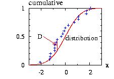 The test calculates the maximum absolute deviation from the cumulative
of the data compared to the cumulative of the distribution we think that
the data come from:
The test calculates the maximum absolute deviation from the cumulative
of the data compared to the cumulative of the distribution we think that
the data come from:
D = max ( | Cdata(x) − F(x) |
)
with Cdata(x) is the cumulative of the data calculated using
vec_cumulative.
F(x) is the cumulative of the distribution.
x varies from +∞ to −∞.
The biggest flaw of this method is that it considers only one data
to calculate D. And D, by definition of F(x), varies from 0 to 1, usually
only the data in the middle of the x range are considered.
The greatest advantage is that we can easily approximate the confidence for this value
of D (which itself has not a lot of interest):
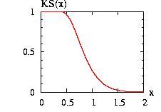
confidence = KS (
(N0.5+0.12+0.11 N-0.5) D
)
with N = number of data and
KS(x) = 2 ∑j (−1)j−1
exp(−2 j2x2)
and j varies from 1 to +∞. If we plot this function, we observe
that the it varies quickly to zero if x > 1.5.
In the formula for the confidence, for big enough value of N we have:
confidence ≈ KS( N0.5 D )
For large N, D ∝ 1/N if the data comes from the distribution,
and D ∝ cst otherwise. Therefore the confidence will tend to 1
for the first case and 0 for the second.
This formula for the confidence works only
if the parameters of the distribution have not been calculated using the data.
If you need to do so, which is the common case, you should divide your
data in two, and use the first part to fit and calculate the
parameters of the distribution, and use the second part of the data
to calculate the goodness of the fit.
The syntax of the static function included in the the class Fit is:
| vector <double> KS_Test(Distribution* dist,vector <double> data) |
|
Return a vector= {D,confidence} |
Example of program:
// Example KS_Test.cpp download
#include "LOPOR.hpp"
using namespace LOPOR;

int main( )
{
    try
    {
        std::vector <double>  vecX,vecY,data,results;

        Normal dist;            // define the distribution
        dist.setParameter(0,1);  // define parameters
        print("data   from   :",dist.information( ));   // display information

        data=dist.ranVector(20);  // random sampling 20 elements
        results=Fit::KS_Test(&dist,data);
        vec_print(results,"20 elements: D_KS, confidence");

        data=dist.ranVector(200);  // random sampling 100 elements
        results=Fit::KS_Test(&dist,data);
        vec_print(results,"200 elements: D_KS, confidence");

        data=dist.ranVector(2000);  // random sampling 1000 elements
        results=Fit::KS_Test(&dist,data);
        vec_print(results,"2000 elements: D_KS, confidence");
    }
catch (const LOPOR::Error& error) { error.information( ); }
return 0;
}
And the output of the program is:
data   from   : LOPOR::Normal(0,1)
#   i=      20 elements: D_KS, confidence
     0       0.199178
     1        0.36631
#   i=      200 elements: D_KS, confidence
     0      0.0551472
     1       0.565521
#   i=      2000 elements: D_KS, confidence
     0      0.0130963
     1       0.880654
The confidence can be calculated as:
confidence = Kuiper (
(N0.5+0.155+0.24 N-0.5) D
)
with N = number of data and
Kuiper(x) = 2 ∑j (4 j2 x2 − 1)
exp(−2 j2x2)
and j varies from 1 to +∞.
This formula for the confidence works only
if the parameters of the distribution have not been calculated using the data.
If you need to do so, which is the common case, you should divide your
data in two, and use the first part to fit and calculate the
parameters of the distribution, and use the second part of the data
to calculate the goodness of the fit.
| vector <double> Kuiper_Test(Distribution* dist,vector <double> data) |
|
Return a vector= {D,confidence} |
For an example, see KS_Test.cpp.
Not currently implemented in this version.
Bayes procedure is a powerful tool to estimate our
uncertainties. For an introduction and review see
[Silvia1996] and
[Gelman2000].
We would like to know the number M of balls in a bag.
We take D=5 balls from the bag, we put a mark on them and put them
back in the bag.
Then we take n=10 balls from the bag: i=2 with a mark,
8 without. We use the Bayes theorem:
f(M|X)=l(X|M) π(X)/Normalization
with X=experience: l(X|M)=Hyperbolic(n,D,M).density(i)=likelihood.
The only things that we know about the
prior probability is that there is at least 10+3=13 balls
in the bag. If we call "post"=f.
The program could be:
// LOPOR.hpp include all the headers of the LOPOR library
#include "LOPOR.hpp"

int main( )
{
    try
    {
            // likelihood: l(n,D,M)
        std::vector <double>  likelihood;
        LOPOR::Hypergeometric hypergeometric;
        for(int M=0; M < 500; ++M)
        {
                // l(n,D,M) does not exist if n > M
            if(M < 10) likelihood.push_back(0);
            else
            {
                hypergeometric.setParameter(10,5,M);
                likelihood.push_back(hypergeometric.density(2));
             }
        }

            // prior: at least 10+5-2=13 balls
        std::vector <double>  prior(LOPOR::vec_create(500,1.));
        prior=LOPOR::vec_fill(prior,0,12,0.);

            // posterior: Bayes procedure
        std::vector <double>  post;
        post=LOPOR::vec_multiply(prior,likelihood);
        post=LOPOR::vec_normalize(post);
        LOPOR::vec_print("post.res",post,"posterior");

    }
    catch (const LOPOR::Error& error) { error.information( ); }
    return 0;
}
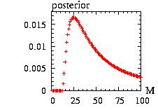 Now you can use a graphic software to plot the file. In
gnuplot we have:
Now you can use a graphic software to plot the file. In
gnuplot we have:
p [0:100] 'post.res' u 1:2 w l
and we get the figure.
The best chance is that the number of balls is around 25 (=5. 10/2)
but we cannot exclude a much bigger number.
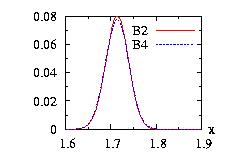 The Bootstrap [Efron1993]
[Davison1997] method is very useful
to calculate uncertainties. It can be seen as a generalization
of the Jackknife techniques. For an example of this last
method, see [Loison2000].
However the Bootstrap is better and easier to apply
than the last procedure.
The Bootstrap [Efron1993]
[Davison1997] method is very useful
to calculate uncertainties. It can be seen as a generalization
of the Jackknife techniques. For an example of this last
method, see [Loison2000].
However the Bootstrap is better and easier to apply
than the last procedure.
The Bootstrap class has only three static
functions. The syntax:
| static vector <double> LOPOR::Bootstrap::ranVector( vector <double> vec) |
|
return a vector of vec.size( ) elements of vec randomly chosen. |
| static vector <double> LOPOR::Bootstrap::meanVector( vector <double> vec, int number_bootstrap) |
|
calcul number_bootstrap averages from the data (vector vec) (non parametric bootstrap). |
| static vector <double> LOPOR::Bootstrap::meanVector( Distribution* d, int number_bootstrap, int nbdata) |
|
calcul number_bootstrap averages from the distribution d. Each bootstrap has nbdata elements (parametric bootstrap). |
If the function is more complicated than a simple average, for example if you have two vectors vec1 and vec2 and want to calculate < vec1.vec2 > − < vec1 > <vec2 > …, you have to write your own program. The figure above uses the results from the program given below. I give several forms for the non parametric and parametric bootstraps when using the Bootstrap class and if the calcul is done without the class.
// Example Bootstrap1.cppdownload
//
// Given = the size of 17 French men.
// Question: what is the size average of all
// French men and our uncertainty about it?

// LOPOR.hpp include all the headers of the LOPOR library
#include "LOPOR.hpp"
using namespace LOPOR;

int main( )
{
    try
    {
        // create a vector of the data
        // vec=size of 17 French men
        std::vector <double>  vec =c2v<double> (1.767,1.778,1.712
                             ,1.683,1.91,1.642, 1.73,1.69,1.81,1.70
                             ,1.75,1.53,1.65,1.78,1.86,1.64,1.5);

        double number_bootstrap=200000;
        std::vector <double>  data, X, Y;

        // 1. Non parametric Bootstrap: form 1: not using the Bootstrap class
        for(int i=0; i <  number_bootstrap; ++i)
            data.push_back( vec_mean( Bootstrap::ranVector( vec ) ) );
        X.clear( ); Y.clear( );

            // How the interval is divided
        X=vec_histogramX(data,1.5,1.9,80,"double");
        Y=vec_histogramY(data,1.5,1.9,80,"double"); // get histogram
        X=vec_middle(X);  //to get the same number oh bins as Y
        Y=vec_normalize(Y);
        vec_print("Bootstrap1.res",X,Y);

        // 2. Non parametric Bootstrap: form 2: using the Bootstrap class
        X.clear( ); Y.clear( ); data.clear( );
        data=Bootstrap::meanVector(vec,number_bootstrap);
        X=vec_histogramX(data,1.5,1.9,80,"double");
        Y=vec_histogramY(data,1.5,1.9,80,"double");
        X=vec_middle(X);
        Y=vec_normalize(Y);
        vec_print("Bootstrap2.res",X,Y);

        // 3. and 4. Parametric Bootstrap
        // If we know that vec follows a normal distribution, for example
        Normal normal;
        normal.setParameter(vec_mean(vec),vec_sigma(vec));

        // 3. Parametric Bootstrap: form 3: : not using the Bootstrap class
        X.clear( ); Y.clear( ); data.clear( );
        for(int i=0; i < number_bootstrap; ++i)
            data.push_back( vec_mean( normal.ranVector( vec.size( ) ) ) );
        X=vec_histogramX(data,1.5,1.9,80);
        Y=vec_histogramY(data,1.5,1.9,80);
        X=vec_middle(X);
        Y=vec_normalize(Y);
        vec_print("Bootstrap3.res",X,Y);

        // 4. Parametric Bootstrap: form 4: using the Bootstrap class
        X.clear( ); Y.clear( ); data.clear( );
        data=Bootstrap::meanVector(&normal,number_bootstrap,vec.size( ));
        X=vec_histogramX(data,1.5,1.9,80);
        Y=vec_histogramY(data,1.5,1.9,80);
        X=vec_middle(X);
        Y=vec_normalize(Y);
        vec_print("Bootstrap4.res",X,Y);
    }
    catch (const Error& error) { error.information( ); }
    return 0;
}
The figure above was plotting using the files "Bootstrap2.res" and "Bootstrap4.res". The second column is using as the x coordinates, the third at the y coordinates.
The class Correlations.hpp has several static functions to estimate correlations between data.
We have two vectors X and Y with N data each
and we would like to estimate the correlations
between them. If we calculate the vectors RankX and RankY which are the rank
for each xi we can define the Spearman coefficient:
rS = ∑i rxi ryi
/ ( ∑i rxi2
∑i ryi2 )0.5
with rxi = RankXi − Mean(RankX) and
ryi = RankYi − Mean(RankY).
The sum runs on the N data.
rS varies from −1 to +1. A value closes to −1 or +1
means that the variables are highly negatively or positively correlated respectively.
The statistical significance can be estimated using.
t = rS ( N − 2 )0.5 /
( 1 − rS2 )0.5
which is distributed approximately as a Student's distribution
with N − 2 degrees of freedom. The confidence can be estimated
using the cumulative of the Student distribution.
The syntax is:
| static vector <double> Correlations::Spearman(vector <double> X, vector <double> Y) |
|
X and Y are the data. |
Example of program:
// Example Spearman.cpp

#include "LOPOR.hpp"
using namespace LOPOR;

int main( )
{
    try
    {
        std::vector<double> X, Y;

        // create a vector X
        Gamma gamma;
        gamma.setParameter(2,1);
        X=gamma.ranVector(30);

        // create a correlated vector Y => big rS
        Normal normal;
        normal.setParameter(0,1);
        Y=vec_add( vec_exp(X) , normal.ranVector(30));

        vec_print(Correlations::Spearman(X,Y),"Correlated: rS, %confidence=");

        // create an uncorrelated vector Y => small rS
        Y=normal.ranVector(30);

        vec_print(Correlations::Spearman(X,Y),"Uncorrelated: rS, %confidence=");
    }
    catch (const Error& error) { error.information( ); }
    return 0;
}
And the output of the program is :
#   i=      Correlated: rS, %confidence=
     0       0.849166
     1              1
#   i=      Uncorrelated: rS, %confidence=
     0     -0.0785317
     1       0.660012
We have two vectors X and Y with N data each
and we would like to estimate the correlations
between them.
We can use Kendall's tau to estimate this correlation. The procedure is very similar
to the one for Spearman's coefficient but what is considered here is just
if a value compared to another data has the same rank (0), a lower rank (−1) or
a bigger rank (+1). The point is to consider all possible pairs in x and y.
If we define:
Then τ can be calculated using:
τ = ( Concordant − Discordant ) /
( (Concordant+Discordant+Tied_x)*
(Concordant+Discordant+Tied_y) )0.5
τ varies from −1 to +1. A value closes to −1 or +1
means that the variables are highly negatively or positively correlated respectively.
The statistical significance can be estimated because τ is
distributed as a Normal's distribution with zero mean (μ=0)
and a variance
στ = ( 4 N + 10 ) / (9 N2-9 N )
if there is no correlation.
The syntax is:
| static vector <double> Correlations::Kendall(vector <double> X, vector <double> Y) |
|
X and Y are the data. |
Example of program:
// Example Kendall.cpp

#include "LOPOR.hpp"
using namespace LOPOR;

int main( )
{
    try
    {
        std::vector<double> X, Y;

        // create a vector X
        Gamma gamma;
        gamma.setParameter(2,1);
        X=gamma.ranVector(30);

        // create a correlated vector Y => big tau
        Normal normal;
        normal.setParameter(0,1);
        Y=vec_add( vec_exp(X) , normal.ranVector(30));

        vec_print(Correlations::Kendall(X,Y),"Correlated: tau, %confidence=");

        // create an uncorrelated vector Y => small tau
        Y=normal.ranVector(30);

        vec_print(Correlations::Kendall(X,Y),"Uncorrelated: tau, %confidence=");
    }
    catch (const Error& error) { error.information( ); }
    return 0;
}
And the output of the program is:
#   i=      Correlated: tau, %confidence=
     0       0.714943
     1    2.88031e-08
#   i=      Uncorrelated: tau, %confidence=
     0     -0.0528736
     1       0.681554
We can observe that the results are very similar to that the
ones given by the
Spearman method. The confidence applies only for the uncorrelated
series. This fact explains the small results for the correlated
series (first case).
Autocorrelation appears when you produce a Markov chain.
In a Markov chain the value xt+1 depends of xt
and therefore the two values are not independent. The objective of this class is
to calculate how many step t between two value you need to have two
"independent" values. The Autocorrelation τ is estimated by calculating
the autocorrelation function Γ(t):
Γ(t)= ∑i (<A(i)A(i+t)> − <A(t)>2)
/ (<A(i)2> − <A(t)>2)
then τ using:
τ = 1 + 2 ∑0τf Γ(t)
with τf is the value of t where Γ=0.01 .
The error Δτ on τ can be estimated using:
Δτ = (τ−1) ( 2 (2 τf + 1)/Nt )1/2
with Nt is the length of the serie. For more information you can
refer to [Loison2000].
| static vector<double> Autocorrelation(const vector<double> x, vector<double>& gamma,const int t_gamma=100); |
|
x is the vector with the data. |
The key point is that you should always plot the Γ function to check if the calcul of
τ is correct. Look at the figure below (the program to generate the figures could be
found here:
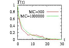 In the first case there is not enough Monte Carlo steps to produce a smooth curve
and the result given by the class is τ= 90.5014 ± 103.089. In the second case the
curve is much smoother and the correct result is tau= 10.5856 ± 0.0986897
In the first case there is not enough Monte Carlo steps to produce a smooth curve
and the result given by the class is τ= 90.5014 ± 103.089. In the second case the
curve is much smoother and the correct result is tau= 10.5856 ± 0.0986897
The class Time.hpp has several static functions to get some forecast
and to calculate some statistics about errors:
| static vector <double> Time::LinearMA(vector <double> X, int N) |
|
X are the initial data. |
Example of program:
// Example Time_Linear1.cppdownload

// LOPOR.hpp include all the headers of the LOPOR library
#include "LOPOR.hpp"
using namespace LOPOR;

int main( )
{
    try
    {
        std::vector<double> X, F;

        X=c2v<double>(1211,1543,1654,1432,1254,1624,1349,1824,1743,1632,1645);

        // Calculate F using the average of 2 elements
        F=Time::LinearMA(X,2);

        // print results
        vec_print(X,F,vec_sous(X,F),"    data,    Forecast,      Errors");

        // accuracy of forecasting
        vec_print(Time::Stat_Errors(X,F,2),"Accuracy of forecasting: MAE,MSE,SE,MAPE");

        // to plot the figure
        vec_print("dataX.res",X);
        vec_print("dataF.res",F);
    }
    catch (const Error& error) { error.information( ); }
    return 0;
}
And the output of the program is:
#   i=          data,    Forecast,      Errors
     0           1211           1211              0
     1           1543           1543              0
     2           1654           1377            277
     3           1432         1598.5         -166.5
     4           1254           1543           -289
     5           1624           1343            281
     6           1349           1439            -90
     7           1824         1486.5          337.5
     8           1743         1586.5          156.5
     9           1632         1783.5         -151.5
    10           1645         1687.5          -42.5
    11                        1638.5        -1638.5
#   i=      Accuracy of forecasting: MAE,MSE,SE,MAPE
     0        199.056
     1        48687.8
     2         73.551
     3        12.7493
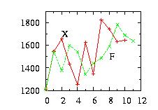
The figure is made using the files 'dataX.res' and 'dataF.res'.
| static vector <double> Time::ExpMA(vector <double> X, double α, int N0, int F0) |
|
X are the initial data. |
Example of program:
// Example Time_Exp1.cppdownload

// LOPOR.hpp include all the headers of the LOPOR library
#include "LOPOR.hpp"
using namespace LOPOR;

int main( )
{
    try
    {
        std::vector<double> X, F;

        X=c2v<double>(1211,1543,1654,1432,1254,1624,1349,1824,1743,1632,1645);

        // Calculate F using the average of 2 elements
        F=Time::ExpMA(X,0.2);

        // print results
        vec_print(X,F,vec_sous(X,F),"    data,    Forecast,      Errors");

        // accuracy of forecasting
        vec_print(Time::Stat_Errors(X,F,2),"Accuracy of forecasting: MAE,MSE,SE,MAPE");

        // to plot the figure
        vec_print("dataX.res",X);
        vec_print("dataF.res",F);
    }
    catch (const Error& error) { error.information( ); }
    return 0;
}
And the output of the program is:
#   i=          data,    Forecast,      Errors
     0           1211           1211              0
     1           1543           1211            332
     2           1654         1277.4          376.6
     3           1432        1352.72          79.28
     4           1254        1368.58       -114.576
     5           1624        1345.66        278.339
     6           1349        1401.33       -52.3286
     7           1824        1390.86        433.137
     8           1743        1477.49         265.51
     9           1632        1530.59        101.408
    10           1645        1550.87        94.1262
    11                        1569.7        -1569.7
#   i=      Accuracy of forecasting: MAE,MSE,SE,MAPE
     0        199.478
     1        57633.1
     2         80.023
     3        12.1528
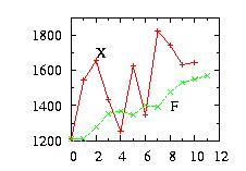
The figure is made using the files 'dataX.res' and 'dataF.res'.
Example of program:
// Example Time_Wiener1.cppdownload

#include "LOPOR.hpp"
using namespace LOPOR;

int main( )
{
    try
    {
        std::vector<double> S, Wiener, histoX, histoY;

        Normal normal;
        normal.setParameter(0.05,0.15);

        // S = 100 exp( Normal(0.05,0.15) )
        Wiener=normal.ranVector(1000000);
        S=vec_multiply(vec_exp(Wiener),100);
        print("mean=",vec_mean(S),"sigma=",vec_sigma(S));

        // histogram
        histoX=vec_histogramX(S,50,200,50,"double",3);
        histoY=vec_histogramY(S,50,200,50,"double",3);
        vec_print("histo.res",vec_middle(histoX),vec_normalize(histoY));

    }
    catch (const Error& error) { error.information( ); }
    return 0;
}
And the output of the program is:
mean= 106.314 sigma= 16.0205
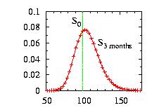
The figure is made using the file 'histo.res' using the second column
for the abscissa and the third for the ordinate.
| static vector <double> Time::Stat_Errors(vector <double> X, vector <double> F, int N0) |
|
X are the initial data. |
Examples of programs in Time_Linear1.cpp and Time_Exp1.cpp.
The class Vector.hpp has various global functions (under the LOPOR namespace) to analyze the data.
The Statistics concerning the vectors (included in the Vector
class defined below) are accessible below:
vec_absDeviation,
vec_histogramY,
vec_histogramX,
vec_max,
vec_max_i,
vec_meanExcess,
vec_meanQuantile,
vec_min,
vec_min_i,
vec_norm,
vec_sigma,
vec_variance,
For an example of program using these functions see the example in the Bootstrap class
Principal component analysis (PCA) involves a mathematical procedure
that transforms a number of (possibly) correlated variables into a
(smaller) number of uncorrelated variables called principal components.
The first principal component accounts for as much of the variability in
the data as possible, and each succeeding component accounts for as much
of the remaining variability as possible.
It has a very wide application to various field, from physics to
genetic [Cavalli-Sforza1996].
We will use principally this method to generate random number
when their distributions are correlated
(see NormalMultiPCA).
It consists to calculate the eigenvalues and the corresponding
eigenvectors to try to understand the most important directions.
One static function include in the MathFunction.hpp
class provide an implementation of the method:
|
static vector<vector<double> >
MathFunctions::matrix_PCA( vector<vector<double> > correlations, vector<double> eigenvalues, vector<vector<double> > eigenvectorsT ) |
|
Return the matrix WPCA=eigenvectors.Λ
with Λ = matrix which elements different of 0 are the
eigenvalues λi on the diagonal. |
The matrix WPCA which is returned
is useful if we want to get N (W.size())
random numbers from a correlated normal distribution
(see NormalMultiPCA).
Example of program:
// Example PCA.cpp
// calculate the principal components for
// a matrix correlation

#include "LOPOR.hpp"
using namespace LOPOR;

int main( )
{
    try
    {
        // matrix
        // | 1   0.1   0.2 |
        // | 0.1   1   0.9 |
        // | 0.2  0.9   1  |
        std::vector<std::vector<double> > correlations=
        c2m( c2v(1.,0.1,0.2), c2v(0.1,1.,0.9), c2v(0.2,0.9,1.));

        matrix_print(correlations,"correlations matrix");
        print( );

        // define eigenvalues and eigenvectors transposed
        std::vector<double> eigenvalues;
        std::vector<std::vector<double> >  eigenvectorsT;
        std::vector<std::vector<double> >  W_PCA;

        W_PCA=MathFunctions::matrix_PCA(correlations,eigenvalues,eigenvectorsT);

        // print results
        vec_print(eigenvalues,"eigenvalues");
        print( );
        matrix_print(eigenvectorsT,"eigenvectorsT");
        print( );
    }
    catch (const Error& error) { error.information( ); }
    return 0;
}
And the output is:
#matrix:  correlations matrix
     1    0.1    0.2
   0.1      1    0.9
   0.2    0.9      1

#   i=      eigenvalues
     0    1.94762
     1   0.958054
     2  0.0943231

#matrix:  eigenvectorsT
0.219038 0.683983 0.695838
0.972429 -0.211519 -0.0981894
-0.0800231 -0.69816 0.711455
We observe that the first direction (0.219038,0.683983,0.695838) explains 1.94762/3. = 65% of the matrix correlation, the second (0.972429,-0.211519,-0.0981894) explains 0.958054/3. = 32%, and the third direction (-0.0800231,-0.69816,0.711455) only 0.0943231/3.=3%. This is due to the strong correlation (0.9) between the second and the third initial directions in the matrix correlations.
The class Global.hpp has various global functions and variables.
| ERROR |
|
The numerical errors ERROR depend of the computer/system that you use. It is principally used to convert a double to an integer. For example, the function c2floor(x) is defined as floor(x+ERROR). |
| PI and Pi |
|
PI=Pi=3.14159265358979323… |
|
double c2d(T x) |
|
Convert a type T to a double |
|
int c2floor(double d) int c2floor(double d,int max) |
|
To take account of the possible error by the computer. Indeed
numerically 1 could be coded as 1.0000000000000003 or
0.9999999999999997 . This happens often if you do some operations. If you use
static_cast <int>, you will get 1 and 0 for the
two previous examples.
The function is defined as
floor(d+ERROR).
For example if ERROR=10-13: |
|
int c2i(T x) |
|
Convert a type T to an
integer = static_cast <int> ( ). |
| vector<vector < T1 > > c2m(vector < T1 > vec1,vector < T1 > vec2, …. ) |
|
Template function to convert
until 30 elements to a matrix (vector<vector>)
=c2v(vec1, vec2,…). For example: |
| string c2s(T x) |
|
Template function to convert a type T to a string. For example: |
| string c2s(vector<T> vec) |
|
Template function to convert a vector of type T to a string: {vector[0],vector[1],…}. For example: |
| vector < T1 > c2v(T1 x1,T1 x2, …. ) |
|
Template function to convert
until 30 elements to a vector. For example: |
| vector < T1 > c2vII(int num, T2 x, …) |
|
Same as c2v but the number of
arguments is no more limited.
Template function to convert num elements of the type T2 to a vector of type T1 elements. For example: |
|
double Log (T1 a) |
|
check if a > 0 and return log(a). T1 can be either a double or an int. Useful to include results from Mathematica® software. |
|
T MAX(T a,T b) T Max(T a,T b) T MAX(T a,T b, Tc) T Max(T a,T b,T c) |
|
return the maximum(a,b) |
|
T MIN(T a,T b) T Min(T a,T b) |
|
return the minimum(a,b) |
|
T1 power
(T1 a, int p=2) double power (T1 a, double p) |
|
return ap if p is an integer |
|
T1 Power (T1 a, int p) double Power (T1 a, double p) |
|
Same as the function power: return ap. Useful to include results from Mathematica® software. T1 can be either a double, an int or the string "E". In this last case Power("E",3)=exp(3). |
|
void print
( a , b, c, d, e…) |
|
Print the variable a, b, … |
| void print_file (string filename, a, b, c … ) |
|
Print the variable a, b, c … in the file filename. |
|
void print_precision(int precision)
|
|
set the precision of standard output. Equivalent to |
|
T sign (T a) |
|
return -1 if a < 0 and +1 otherwise |
|
double Sqrt (T1 a) |
|
check if a > 0 and return a1/2. T1 can be either a double or an int. Useful to include results from Mathematica® software. |
|
T heaviside (T a) T Heaviside (T a) |
|
return 0 if a ≤ 0 and +1 otherwise |
The class Vector.hpp has various global functions (under
the LOPOR namespace) concerning the vectors and
the matrix vector<vector<double> >.
The other
global functions are in the Global class.
We note that this last class is automatically included if
you include the Vector class.
To create a vector from data you should use the function c2v (convert to vector) given in the class Global. Otherwise you can create a vector filled by constant like {1,1,1,…} or with a regular increment like {0,2,4,6,…} using the function vec_create given below. For all other functions (but vec_print) you give a vector and the function returns another vector after doing some manipulation on the elements. The vector(s) given to the function is (are) always defined as const. Moreover the type T, T1 … means that the function is a template.
|
vector < T > vec_abs(vector < T > vec) |
||||||||
|
Return a vector {abs(vec[i])} |
||||||||
|
double vec_absDeviation(vector < T1 > vec) |
||||||||
|
return the sample absolute deviation = |
||||||||
|
vector < T1 > vec_add(vector < T1 > vec1, T2
constant) vector < T1 > vec_add(vector<T1 > vec1, vector < T2 > vec2) |
||||||||
|
Add the constant to the vector vec1. |
||||||||
|
vector < T1 > vec_append(vector<T1 > vec1,
T2 value) vector < T1 > vec_append(vector<T1 > vec1, vector < T2 > vec2) |
||||||||
|
return a new vector {vec1,value}. |
||||||||
|
vector <double> vec_c2d(vector<T > x) |
||||||||
|
Convert a vector of a type T to a double |
||||||||
|
vector <int> vec_c2i(vector<T > x) |
||||||||
|
Convert a vector of a type T to an
integer using static_cast<int>( ) function. |
||||||||
| vector <int> vec_c2floor( std::vector <double> vec) | ||||||||
|
Convert a vector of double to a vector of integer using the c2floor( ) function. |
||||||||
|
vector <double> vec_c2s(vector<T > vec) |
||||||||
|
Convert a vector of a type T to a string "{vec[0],vec[1],…}" |
||||||||
| vector < T1 > vec_create(int n, T1 ini=0, T1 add=0) | ||||||||
|
create a vector of the type T1 filled with n
elements equal to {ini,
ini+add,…}. |
||||||||
| vector < T1 > vec_create2(T1 ini, T1 fin,T1 δ=1) | ||||||||
|
create a vector of the type T1 filled with {ini,ini+δ,…,ini+n*δ≤fin} |
||||||||
| vector < T1 > vec_create3(T1 ini, T1 fin,int n=10) | ||||||||
|
create a vector of the type T1 filled with n+1 elements.
With δ=(fin-ini)/n: {ini,ini+δ,…,ini+(n-1)*δ,fin} |
||||||||
| vector <double> vec_cumulative(vector <double> vecX) | ||||||||
|
return a cumulative vector between 0 and 1, identical to
vec_create(vecX.size( ),1./vecX.size( ),
1./vecX.size( )). |
||||||||
| vector <double> vec_cumulative_histo(vector <double> vecX) | ||||||||
|
return a cumulative vector between 0 and 1.
Each element of vecX must be positive. |
||||||||
|
vector <double>
vec_derivative(vector <double> vec, vector <double> X) vector <double> vec_derivative(vector <double> vec, double dx=1) |
||||||||
|
return the derivative vector. The derivative is calculated using:
vec_derivative(vec,X)={1,2,4,6,8,9} vec_derivative(vec,1)={1,2,4,6,8,9} vec_derivative(vec)={1,2,4,6,8,9} |
||||||||
| vector < T1 > vec_divide(vector<T1 > vec1, T2 constant) | ||||||||
|
Divide the vector by the constant different of zero. |
||||||||
| vector < T1 > vec_divide (vector < T1 > vec1, vector<T2 > vec2) | ||||||||
|
Divide the two vectors:
vec_divide[i]=vec1[i]/vec2[i]. |
||||||||
| vector <double> vec_exp(vector<T1 > vec) | ||||||||
|
Apply the exponential function to each element of the
vector. |
||||||||
|
vector < T1 > vec_fill(vector<T1 > vec, T2 value) vector < T1 > vec_fill(vector<T1 > vec, int pos1, int pos2, T2 value) |
||||||||
|
return a vector where the elements vec[pos1] to vec[pos2]
are replaced by static_cast <T1> (value).
If no positions are given, all elements are replace by value.
This last case corresponds to the function
vec_create(vec.size(),value) |
||||||||
|
vector < T1 > vec_func(T1 function(T2 x),vector<T2 > vec) |
||||||||
|
return a vector {func(vec[0]),func(vec[1]),…) |
||||||||
|
vector < T1 > vec_func(T1 function(std::vector<T2> para),vector<vector<T2 > > vec) |
||||||||
|
return a vector {func(vec[0]),func(vec[1]),…) |
||||||||
| vector <double> vec_group(vector < T1 > vec, int ngroup) | ||||||||
|
return a vector of the size=vec.size(
)/ngroup. The
elements are the average of ngroup
elements. For example, if ngroup=3: |
||||||||
| vector <double> vec_histogramY(vector < T > vec, double xmini, double xmaxi, int n, string type="double",int border=0) | ||||||||
|
Return the histogram of the vector vec. The interval
[xmini,xmaxi] is divided in n or n+1 if the type is
"double" or "int".
The option border=0, 1, 2, or 3 excludes or includes the data outside the range.
For example, the previous example gives:
vecX=vec_histogramX(vec,0,1,10); vecY=vec_histogramY(vec,0,1,10); vec_print(vec_middle(vecX),vecY); you can also use: vec_histogram_print(vec,0,1,10) |
||||||||
|
vector <double> vec_histogramX(vector < T > vec,
double xmini, double xmaxi, int n, string
type="double",int border=0) vector <double> vec_histogramX( double xmini, double xmaxi, int n, string type="double") |
||||||||
|
Return a vector composed of the extremity of each division of the X coordinate. See vec_histogramY for more details. The option border has no effect. The vector vec is not important also. For example, if min=0, max=3, n=3
The size of vec_histogramX = the size of vec_histogramY.size( )+1.
To print the result of the histogram of a vector vec
you should use the function vec_middle.
For example with vec a vector with data: |
||||||||
|
void vec_histogram_print(vector < T > vec,
double xmini, double xmaxi, int n, string
type="double",int border=0) void vec_histogram_print(string file,vector < T > vec, double xmini, double xmaxi, int n, string type="double",int border=0) |
||||||||
|
Print on the screen or in the file "file"
the result of the histogram. It is identical at : For the options see vec_histogramY. |
||||||||
|
vector < T1 > vec_insert(vector < T1 > vec1,
T2 value, int n=vec1.size( )) vector < T1 > vec_insert(vector<T1 > vec1, vector < T2 > vec2, int n=vec1.size( )) |
||||||||
|
insert the value or the vector vec2 at the position
n in the vec1. If n=vec1.size( ), this function is
identical to vec_append. |
||||||||
| vector <double> vec_inverse(vector<T1 > vec) | ||||||||
|
Return −vec; |
||||||||
| vector <double> vec_log(vector<T1 > vec) | ||||||||
|
Apply the logarithm function to each element of the
vector. |
||||||||
| T1 vec_max(vector < T1 > vec) | ||||||||
|
return the maximum value.
Example: vec={1.,3.,0.,2.,3.} |
||||||||
| int vec_max_i(vector < T1 > vec) | ||||||||
|
return the integer position i of the maximum value.
For multiple solutions return the first occurrence.
Example: vec={1.,3.,0.,2.,3.} |
||||||||
| double vec_mean(vector < T1 > vec) | ||||||||
|
Calcul the mean of the vector |
||||||||
| double vec_mean(vector < T1 > X, vector < T2 > histo) | ||||||||
|
Calcul the mean of the vector X if each element of X has its corresponding probability
stocked in the vector histo |
||||||||
| vector <double> vec_meanExcess(vector < T1 > vec) | ||||||||
|
Calcul the mean for each element i as: |
||||||||
|
double vec_meanQuantile(vector < T1 >
vec, T1 vecmin) |
||||||||
|
Calcul the mean of the vector |
||||||||
| vector <double> vec_middle(vector < T1 > vec) | ||||||||
|
return a vector of the size=vec.size( )−1. The
elements are the average of two following elements:
{(vec[0]+vec[1])/2,(vec[1]+vec[2])/2,…,(vec[n−1]+vec[n])/2}.
Useful with vec_histogramX( ). |
||||||||
| T1 vec_min(vector < T1 > vec) | ||||||||
|
return the minimum value.
Example: vec={1.,3.,0.,2.,3.} |
||||||||
| int vec_min_i(vector < T1 > vec) | ||||||||
|
return the integer position i of the minimum value.
For multiple solutions return the last occurrence.
Example: vec={1.,3.,0.,2.,3.} |
||||||||
| vector < T1 > vec_multiply(vector<T1 > vec1, T2 constant) | ||||||||
|
Multiply the vector by the constant. |
||||||||
| vector < T1 > vec_multiply (vector < T1 > vec1, vector<T2 > vec2) | ||||||||
|
Multiply the two vectors:
vec_multiply[i]=vec1[i].vec2[i]. |
||||||||
|
vector <double> vec_normalize(vector<T1 > vec,
double norm) vector < T1 > vec_normalize(vector<T1 > vec) |
||||||||
|
Calcul the norm (sum of elements) and divide each
element by the norm.
Throw an error if norm=0. |
||||||||
| double vec_norm(vector < T1 > vec) | ||||||||
|
Calcul the norm of the vector = sum of all elements. |
||||||||
| vector < T1 > vec_NULL( ) | ||||||||
|
create a vector of the type T1 without elements. Example: vec_NULL <int> ( ). Can also be created using vec_create(0,0) or using c2v <int> ( ). |
||||||||
|
vector < T1 > vec_polynome(vector<T1 > vec, vector<T1 > coeff) vector < T1 > vec_polynome(vector<T1 > vec, T1 coeff0) vector < T1 > vec_polynome(vector<T1 > vec, T1 coeff0, T1 coeff1) … |
||||||||
|
vector coeff=
{coeff0,coeff1,coeff2,…} |
||||||||
|
vector < T1 > vec_power
(vector < T1 > vec, int power) vector <double> vec_power (vector < T1 > vec, double power) |
||||||||
|
Calcul the vec[i]^power for each element vec[i] |
||||||||
|
void vec_print
(vector < T > vec {,vec2,vec3,vec4},string s="") |
||||||||
|
Print the vector under the form "i vector[i]". If the string
s is defined, the first line will be
"#i string s", otherwise no comment is printed.
The vectors {vec2, vec3,vec4} are optional.
| ||||||||
|
void vec_print_1
(vector < T > vec ,string s="",int precision=-1) |
||||||||
|
Print the vector under the form "s vector[0] vector[1] …"
on one line. | ||||||||
| void vec_print (string filename,vector < T > vec{,vec2,vec3,vec4},string s="") | ||||||||
|
Print the vector under the form "i vector[i]" in the file filename. If the string s is defined the first line will be "#i string s", otherwise no comment is printed. The vectors {vec2, vec3,vec4} are optional. |
||||||||
|
vector < int > vec_rank1(vector<T > vec) vector < int > vec_rank2(vector<T > vec) vector < double > vec_rank3(vector<T > vec) |
||||||||
|
Return a vector with the ranks of the elements.
If some elements are equal, assign |
||||||||
| vector < T > vec_remove(vector<T > vec, int n) | ||||||||
|
remove the element at the position n, i.e. the n+1 element
(the vector begins at 0). |
||||||||
| vector < T > vec_remove(vector<T > vec, int ini, int fin) | ||||||||
|
remove the elements between the position ini (included)
and the positions fin (excluded). |
||||||||
| vector < T > vec_replace(vector<T > vec1, vector<T > vec2, int j=0) | ||||||||
|
Replace the elements of vector vec1 by the elements of vec2 from the position j (included) |
||||||||
| double vec_sigma(vector < T1 > vec) | ||||||||
|
variance1/2 |
||||||||
| double vec_sigma(vector < T1 > X, vector < T2 > histo) | ||||||||
|
variance(X,histo)1/2 |
||||||||
| vector < T > vec_sort(vector<T > vec) | ||||||||
|
Sort the elements of vec and return a new vector. |
||||||||
|
vector < T1 > vec_sous(vector < T1 > vec1, T2
constant) vector < T1 > vec_sous(vector<T1 > vec1, vector < T2 > vec2) |
||||||||
|
SoustractAdd the constant to the vector vec1. |
||||||||
| vector < T > vec_thresholdM(vector < T > vec, value) | ||||||||
|
return a vector composed of all vec[i] < value; |
||||||||
| vector < T > vec_thresholdP(vector < T > vec, value) | ||||||||
|
return a vector composed of all vec[i] ≥ value; |
||||||||
| vector < T > vec_truncation(vector < T > vec, int ini, int fin) | ||||||||
|
return a vector composed of
{vec[ini],vec[ini+1],…,vec[fin−1]}: ini included,
fin excluded. |
||||||||
| vector < vector<T> > vec_XYZ(vector < vector<T> > XYZ) | ||||||||
|
XYZ={X,Y,…} with X={x0,x1,…},
Y={y0,y1,…}, … |
||||||||
| double vec_variance(vector < T1 > vec) | ||||||||
|
Calcul the variance of the vector = sum of all
(elements−vec_mean( ))2/(number of elements−1) |
||||||||
| double vec_variance(vector < T1 > X, vector < T2 > histo) | ||||||||
|
Calcul the variance of the vector X if each element of X has its corresponding probability
stocked in the vector histo |
| vector < T1 > matrix_append(vector<vector< T1 > > matrix, vector< T1 > vec) | ||||
|
Append the vector to the matrix.
Example:
matrix={{1,2},{3,4}}, vec={5,6} |
||||
| vector < T1 > matrix_append(vector<vector< T1 > > matrix1, vector<vector< T1 > > matrix2) | ||||
|
Append the matrix2 to the matrix1.
Example:
matrix1={{1,2},{3,4}}, matrix2={{5,6}} |
||||
|
string matrix_c2s(vector<vector < double > >& matrix) |
||||
|
Convert a matrix of a type T to a string |
||||
|
string matrix_c2s_1(vector<vector < double > >& matrix) |
||||
|
Convert a matrix of a type T to a string |
||||
| void matrix_clear(vector<vector < double > >& matrix) | ||||
|
Update and clear the matrix matrix |
||||
| vector<vector < T1 > > matrix_create(int n_lines, int n_col, T1 value=0) | ||||
|
Create a matrix (n_lines*n_col), initialized with value.
Example: |
||||
| vector<vector < vector < T1 > > > matrix3_create(int n_lines, int n_col, int n_col2, T1 value=0) | ||||
|
Create a matrix (n_lines*n_col*n_col2), initialized with value.
Example: |
||||
|
void matrix3_print
(vector<vector < vector<T> > > matrix ,string s="") |
||||
|
Print the matrix. | ||||
| void matrix_S_eigen(vector<vector < double > > matrix, vector < double > eigenvalues, vector<vector < double > > eigenvectors) | ||||
|
The matrix matrix must be
symmetric. Only the upper right corner
of the matrix is considered. |
||||
| void matrix_size_check(vector<vector < double > > matrix) | ||||
|
check if the matrix is of the type M*N, i.e. if all elements (vector) of the vector matrix, have the same size. |
||||
| void matrix_size_MM_check(vector<vector < double > > matrix) | ||||
|
check if the matrix is of the type M*M |
||||
| vector<vector < T1 > > matrix_inverse(vector<vector < T1 > > matrix ) | ||||
|
create a inverse of a (n*n) matrix using the LU decomposition. Example: SolveLinearEqs.cpp |
||||
| vector < T1 > matrix_matrix(vector<vector< T1 > > matrix1, vector<vector< T1 > >) matrix2 | ||||
|
return the product of matrix1 (n_lines*n_col) by the matrix2 (n_col*n_lines).
Example:
matrix1={{1,2},{3,4}}, matrix2={{2,2},{1,1}} |
||||
| vector<vector < T1 > > matrix_NULL( ) | ||||
|
create a matrix of the type T1 without elements. Example: matrix_NULL <int> ( ). Can also be created using matrix_create<int>(0,0) or using c2v(c2v <int> ( )). |
||||
|
void matrix_print
(vector<vector < T > > matrix ,string s="",int precision=6) |
||||
|
Print the matrix.
| ||||
|
void matrix_print
(string filename, vector<vector < T > > matrix ,string s="",int precision=6) |
||||
|
Print the matrix in the file "filename". | ||||
| vector < T1 > matrix_remove(vector<vector< T1 > > matrix, int n_line) | ||||
|
remove the line n_line+1 (the count begins to 0) of the matrix.
Example:
matrix={{1,2},{3,4}} |
||||
| vector < T1 > matrix_vec(vector<vector< T1 > > matrix, vector< T2 > vec) | ||||
|
Create a vector of n_lines =
product of matrix (n_lines*n_col) by a vector (n_col).
Example:
matrix={{1,2},{3,4}}, vec={5,6} |
||||
| vector < vector<T> > matrix_transposed(vector < vector<T> > XYZ) | ||||
|
XYZ={X,Y,…} with X={x0,x1,…},
Y={y0,y1,…}, … |
This section is devoted to the integration in one dimension for
"smooth enough" functions.
I = ∫ab f(x).dx
For more problematic functions, for example
if only one small
part of the space contributes to the integral, and for
multidimensional integration, see the Monte Carlo section:
Integration, Vegas and
Integration with Normalization.
|
static double MathFunctions::Romberg(double function(const double& ),const double& a, const double& b);
|
| Returns the integration of the function on the interval a,b |
Example of program:
// Example Romberg.cpp
// calcul of the integral of f(x) between a and b

#include "LOPOR.hpp"
using namespace LOPOR;

// function to integrate
double func(const double& x) { return 3.*x*x; }

int main( )
{
    try
    {
        print("ROMBERG=",MathFunctions::Romberg(func,0,2));
        print("exact  =",power(2,3)-power(0,3));
    }
    catch (const Error& error) { error.information( ); }
    return 0;
}
And the output of the program is :
ROMBERG= 8
exact  = 8
Imagine that you want to calculate an integral of the form:
I = ∫AB f(x).dx
with a function f(x). If we know the primitive F of f, we can write:
I = ∫AB d(F(x))
I = ∫F(A)F(B) dy
I = F(B) − F(A) .
Obviously we almost never know the cumulative of the function f.
Now imagine that we know that f is more or less constant on the interval [A,B].
We can simply sampled the interval [A,B] randomly and estimate the integral by:
I = (B − A) <f> ±
(B − A) [<f2> − <f>2]½ / N½
Obviously we cannot apply this method if the interval is infinite. Moreover,
and the first problem is related to it, if the integral is dominated by a small portion of [A,B] the result will be inaccurate. Therefore it is better to use
the method:
I = ∫AB f(x).dx
I = ∫AB f(x)/g(x) . g(x).dx
I = ∫AB f(x)/g(x) .d(G(x))
I = ∫G(A)G(B) f(x(y))/g(x(y)) .dy
I = (G(B) − G(A)) <f/g>(G) ±
(G(B) − G(A)) [<f2/g2>(G)
− <f/g>(G)2]½ / N½
with g a function with G its know primitive, and < >(G) means
the the average is taken along the configurations given by the probability g.
The best choice of the function g(x) is the ones the nearest to f(x) or exactly
of |f(x)| since f(x) can be negative.
It is not difficult to generalize the integral to n dimensions.
In this case, since it is not so easy to find a multivariate distribution
which fit the function f, it is usually easier to use a multiplication
of univariate distributions, one for each variable.
Our simple implementation (the next section introduce a better method)
is:
| static vector <double> MonteCarlo::Integration (double func(const vector<double> & ), vector<Distribution*> dist, double limit=0.001, int NbMC_max=100000) |
|
Return a vector {Integral,error,nb of MC} |
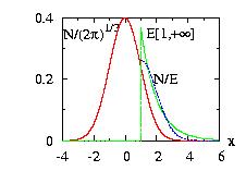
For example imagine that we want to calculate
I = ∫∫1∞ 1/(2 π)
exp(−x2/2 −y2/2) dx dy .
The function f is the product of two normal
Normal(0,1) f(x) and f(y) functions.
We can use the function:
g(x,y)=g(x)*g(y) = e−x*e−y i.e.,
two Exponential(1) functions, to calculate the integral.
It is not the best choices but it will work.
On the figure (y=0) we observe that f/g=N/E is not constant but at least where f=N is
small (x>5) , the function g=E is also small.
The program could be:
// Example Integration1.cpp
// Calcul of the integral of the normal*normal distribution (mean 0, sigma=1)
// between 1 to +oo

#include "LOPOR.hpp"
using namespace LOPOR;

// We want the integral of this function
double func(const std::vector<double>& parameters)
{
    double x=parameters[0];
    double y=parameters[1];
    if(x<1) return 0.;
    if(y<1) return 0.;
    return 1./sqrt(2.*Pi) * exp(-x*x/2.)*1./sqrt(2.*Pi) * exp(-y*y/2.);
}

int main( )
{
    try
    {
        // We want the exponential between 1 to +oo
        // exponential between 0 to +oo
        Exponential expo;
        expo.setParameter(1);

        // exponential between 1 to +oo
        // interval.setParameter(A,B,border=2). With this border
        // the selection is [A,+oo]
        Interval interval;
        interval.setParameter(&expo,1,100,2);

        // Calcul of integral
        std::vector<double> res=MonteCarlo::Integration(func,c2v<Distribution*>(&interval,&interval));
        print("\nThe integral of the normal*normal distribution between 1 to +oo is:");
        print("By Monte Carlo: I =",res[0],"+/-",res[1],"in "+c2s(res[2])+" MC steps");

        // Direct approximation almost exact
        // For the predefined distribution the cumulatives
        // vary from 0 to 1 when the variable varies from -oo to +oo
        // and the tot integral = Ftot.
        Normal normal;
        normal.setParameter(0,1);
        double I_exact=(1.-normal.cumulative(1.))*normal.get_Ftot();
        print("exact result    I =",I_exact*I_exact,"\n");

    }
    catch (const Error& error) { error.information( ); }
    return 0;
}
The integral of the normal*normal distribution between 1 to +oo is:
By Monte Carlo: I = 0.0251558 +/- 6.21674e-05 in 100000 MC steps
exact result    I = 0.0251715
We note that the best function g should be as close as possible to f and the best possible choice is a StepFunction [Loison2004]. For an example of construction see Hasting figure and the corresponding program Hasting1.cpp .
The importance sampling is very useful but we can improve the
integral using the stratified sampling. It consists to divide the
volume dV=dx.dy.… in several disjoint parts. Then it can be proved
that the variance of the average of the results for each part
is less than if we calculate the integral over the whole space
directly.
The Vegas algorithm [Lepage] combine both procedure
(stratified and importance sampling).
One of the flaw of the algorithm is that it uses a kind of
StepFunction as function g. The problem is that
the interval must be finite. Therefore if your interval of integration
is infinite, you should do a change of variable before. Usually y=exp(-x),
or something similar, should work. The syntax is:
| static vector <double> MonteCarlo::Vegas (double func(const vector<double> & ), vector<double> Interval, int NbMC_max=10000,int evaluations=5) |
|
Return a vector {Integral,error,nb of MC} |
If we want calculate the same integral as before:
I = ∫∫1∞ 1/(2 π)
exp(−x2/2 −y2/2) dx dy .
The function f is the product of two normal
Normal(0,1) f(x) and f(y) functions. First we
do the change of variables: X=exp(-x) and Y=exp(-y). We obtain
I = ∫∫e0e−1 1/(2 π)
exp(−log(X)2/2 −log(Y)2/2)/(X.Y) dX dY .
The program could be:
// Example Vegas.cpp
// Calcul of the integral of the normal*normal distribution (mean 0, sigma=1)
// between 1 to +oo

#include "LOPOR.hpp"
using namespace LOPOR;

// We want the integral of this function
double func(const std::vector<double>& parameters)
{
    double x=parameters[0];
    double y=parameters[1];
    return 1./sqrt(2.*Pi) * exp(-log(x)*log(x)/2.)/x*1./sqrt(2.*Pi) * exp(-log(y)*log(y)/2.)/y;
}

int main( )
{
    try
    {
        // With the change of variable X=exp(-x), X varies from 0 to exp(-1)
        std::vector<double> InterX=c2v(0.,exp(-1.));
        std::vector<double> InterY=c2v(0.,exp(-1.));

        std::vector<double> res=MonteCarlo::Vegas( func,c2v(InterX,InterY),50000,2 );
        print("\nThe integral of the normal*normal distribution between 1 to +oo is:");
        print("By Monte Carlo (Vegas): I =",res[0],"+/-",res[1],"in "+c2s(res[2])+" MC steps");

        // Direct approximation almost exact
        // For the predefined distribution the cumulatives
        // vary from 0 to 1 when the variable varies from -oo to +oo
        // and the tot integral = Ftot.
        Normal normal;
        normal.setParameter(0,1);
        double I_exact=(1.-normal.cumulative(1.))*normal.get_Ftot();
        print("exact result            I =",I_exact*I_exact,"\n");

    }
    catch (const Error& error) { error.information( ); }
    return 0;
}
And the output is
The integral of the normal*normal distribution between 1 to +oo is:
By Monte Carlo (Vegas): I = 0.0251713 +/- 4.25293e-07 in 100000 MC steps
exact result            I = 0.0251715
For the same number of MC, the result is better than with the function Integration which gives an error 100 times bigger (≈10−5).
Imagine that you want to calculate an integral of the form:
I = ∫∫∫∫ f(x,y,z,…).g(x,y,z,…).dx.dy.dz.…
/ ∫∫∫∫ g(x,y,z,…).dx.dy.dz.…
In physics, this integral is more common than without normalization, i.e.
denominator.
We admit that the function f(x) is not too much singular, or at least
f and g are singular in the same way. For example, f and g will be not zero only
in a very tiny region (sub-space) of the integration space. In this case the
integration is much more easier with the normalization (the integral in
the denominator) than without. The key point is that we do not need to calculate
the denominator. Indeed we can rewrite the integral like, using for clarity
only one variable:
I = ∫AB f(x). g(x).dx / ∫AB g(x).dx
I = ∫AB f(x) .d(G(x)) / ∫AB d(G(x))
I = ∫G(A)G(B) f(x(y)).dy / ∫G(A)G(B) dy
I = [
(G(B) − G(A)) <f>(G) ±
(G(B) − G(A)) [<f2>(G)
− <f>(G)2]½ / N½
]
/ (G(B) − G(A))
I =
<f>(G) ±
[<f2>(G)
− <f>(G)2]½ / N½
therefore we just have to find a way to simulate configurations following
the probability g(x) without the need to calculate the
integral of g. There is a very easy way to do it, using a Markov process.
From an initial configuration
x0
we found a new configuration {x1} with the
detail balance condition:
g(x0) T(x0 → x1} =
g(x1) T(x1 → x0} .
T is the transition probability between the configuration x0
and x1.
This relation is a consequence of a time invariance
of the integral.
It is not difficult to
generalize this formula for more variables.
The interest of this process is that we can simulate any function g since
the only problem is to find the transition probability T. It is no need to
have a global way to simulate g but only a local way. The price to be paid
is that the configurations will not be independent and therefore the
N½ in the formula above should be replaced by
(N/τ)½ with τ the
autocorrelation time.
There are many ways to find an efficient transition probability T.
The reader is invited to read [Loison2004]
for a complete review of local updates.
In the following we will use the
MetropolisRestricted class.
In the following we give the program to calculate the magnetization of
10 infinite Ising spins with ferromagnetic long range interactions.
The function g can be written as:
g(x0,x1,…)=
exp(∑i ∑j≠i xi xj /temperature)
and the function f is:
f(x0,x1,…)= ∑i xi .
The program:
// Example IntegrationNormalization.cpp
// calculate I=Integral(f.g)/Integral(g) on [-1,1]
// for 10 variables. Correspond to the physical model
// of 10 continuous Ising spins with long range ferromagnetic
// interaction at the temperature T=3;

#include "LOPOR.hpp"
using namespace LOPOR;

// g= x[0]*(x[1]+x[2]+…+x[9])+x[1]*(x[2]+…+x[9])+…
//  -1 <= x <= 1
double g(const std::vector<double>& x)
{
    for(int j=0; j<x.size(); ++j)
        if(x[j]<−1 || x[j] >1) return 0.;

    double res=0.;
    for(int j=0; j<x.size(); ++j)
    for(int i=0; i<x.size(); ++i)
        if(i != j) res += x[i]*x[j];

    return exp(res/(2.*3.));
}

double f(const std::vector<double>& x)
{
    return vec_mean(vec_abs(x));
}

int main( )
{
    try
    {
        // MetropolisRestricted
        // x_ini=(0,0,0,…)
        // delta_ini=(0.5,0.5,…)
        // function g to simulate with Markov Metropolis restricted
        // with 1000 initial steps to reach an configuration in equilibrium
        // and the delta should be updated  (0 at the end of setParameter)
        std::vector<double> x=vec_create(10,0.);
        std::vector<double> delta=vec_create(10,0.5);
        MetropolisRestricted metRes;
        metRes.setParameter(g,x,delta,1000,0);

        // value of delta after the iterations:
        vec_print(metRes.delta,"value of delta after the iterations");

        // MC random number following g:
        // one random number = a vector of 10 random numbers
        // {ran_x0,ran_x1,…,ran_x10}
        int MC=100000;
        std::vector<std::vector<double> > ranX=metRes.ranVector(MC);

        // Apply f for each random number: we have {f_t=1,f_t=2,…,f_t=MC}
        std::vector<double> res=vec_func(f,ranX);


        // Calcul of tau and gamma
        std::vector<double> gamma, tau;
        tau=Correlations::Autocorrelation(res,gamma);

        // print result for tau and gamma (in file "gamma" to plot)
        print("tau=",tau[0]," +/-",tau[1]);
        vec_print("gamma",gamma);

        // Result of integral with error
        double Integral  = vec_mean(res);
        double error_sqr = (vec_mean(vec_power(res,2))
                          -power(vec_mean(res),2))/(c2d(MC)/tau[0]);
        print("The integral =",Integral," +/-",sqrt(error_sqr));

    }
    catch (const Error& error) { error.information( ); }
    return 0;
}
And the output of this program:
#   i=      value of delta after the iterations
     0    1.24416
     1    1.24416
     2    1.49299
     3    1.24416
     4    1.24416
     5    1.24416
     6    1.24416
     7     1.0368
     8    1.49299
     9    1.24416
tau= 10.6722  +/- 0.320789
The integral = 0.551179  +/- 0.00110453
The figure for Γ can be found here.
The class MonteCarlo has one static function that calculate
the Losses:
where N is determined by a frequency distribution and the
individual losses li are determined by the
severity distribution. The two distributions are
independent.
The syntax is:
| static vector <double> MonteCarlo::Losses (Distribution* frequency, Distribution* severity, double limit=0.001, int NbMC_max=100000) |
|
Return a vector {losses,error,nb of MC} with error=sqrt(variance)/(nb of MC). |
Example:
// Example MonteCarlo1.cpp download
//
// Calcul the Losses = Sum_i(l_i)
// where l_i are individual loss events
// and i varies from 1 to N.
// The value N follows a distribution : the frequency
// The values l_i follow another distribution: the severity
// The frequency and the severity are independent
//
#include "LOPOR.hpp"
using namespace LOPOR;

int main( )
{
    try
    {
        // Frequency
        //
        Normal freq;
        freq.setParameter(30,4);

        // Severity
        //
        Lognormal sev;
        sev.setParameter(100,20);

        // calcul stop when: sigma/mean  < limit=0.0002
        // or when: number of Monte Carlo NbMC  > 100000
        // NbMC = nb of time that the sum Sum_i(l_i) is done
        //
        std::vector<double> results;
        results=MonteCarlo::Losses(&freq,&sev,0.0002,100000);

        vec_print(results,"Losses, Sigma, nb of MC=");
    }
    catch (const LOPOR::Error& error) { error.information( ); }
    return 0;
}
And the output is:
#   i=      Losses, Sigma, nb of MC
     0        99.5245
     1      0.0198091
     2          37000
In this section we will treat the partial differential equations
which appear in Option pricing, i.e. the
equation of diffusion of heat:
∂u/∂t = ∂2u/∂x2
the general form of the equation
∂u/∂t = a(x) ∂2u/∂x2
+ a'(x) |∂2u/∂x2|
+ b(x) ∂u/∂x + c(x) u(x) + d(x)
and the general form in presence of
transaction costs of the equation
∂u/∂t = a(x) ∂2u/∂x2
+ a'(x) |∂2u/∂x2|
+ b(x) ∂u/∂x + c(x) u(x) + d(x)
∂u/∂t = ∂2u/∂x2
We can replace the derivatives by:
∂u/∂t = (ui,j+1 - ui,j)/dt
∂2u/∂x2 =
(ui+1,j-2 ui,j + ui-1,j)/dx2
where the x and t spaces are discretized in N steps of dx and Nt steps of dt.
The notation ui,j= u(x=i*dx,t=j*dt).
The equation can be re-written as:
ui,j+1 = ui,j + α (ui+1,j-2 ui,j + ui-1,j)
α = dt/dx2
Conditions: We have the form of u at t=0 (i.e. j=0) : ui,0.
Moreover we need two more conditions at the boundaries for all t, i.e. all j.
There is two choices: the conditions could be on u or on the derivative
∂u/∂x.
If we have the values of ui,0 and the conditions u0,j
and uN,j (the extremities of the x space) it is not difficult to
apply the formula recursively for all j > 0 (i.e. t>0) and i between 1 to N−1. We have to go from the time t=0 (i.e. j=0) to the time t=dt
(i.e. j=1) the equations:
u0,1=u0,0
u1,1 = u1,0 + α (u2,0-2 u1,0 + u0,0)
u2,1 = u2,0 + α (u3,0-2 u2,0 + u1,0)
…
uN-1,1 = uN-1,0 + α (uN,0-2 uN-1,0 + uN-2,0)
uN,1=uN,0
We can apply these formulae for j=1, then for j=2, …
We impose now at the boundaries u0,j at the origin x=0, but
∂u/∂x=f at i=N (x=1) for all j (i.e. all t). f could be a
constant value but also could be a function of u.
We still
have the form of the function at t=0 for all x ui,0.
The equation ∂u/∂t = ∂2u/∂x2
at i=N can be read as:
uN,j+1 = uN,j + α (uN-1,j-2 uN,j + uN+1,j)
and the condition for the derivative ∂u/∂x=f at i=N:
(uN+1,j-uN,j)/dx = f
we can eliminate the fictitious variables uN+1,j to arrive at the
equation:
uN,j+1 = uN,j + α (uN-1,j-2 uN,j + uN,j + f.dx)
Therefore the equations for t=dt read as:
u0,1=u0,0
u1,1 = u1,0 + α (u2,0-2 u1,0 + u0,0)
u2,1 = u2,0 + α (u3,0-2 u2,0 + u1,0)
…
uN-1,1 = uN-1,0 + α (uN,0-2 uN-1,0 + uN-2,0)
uN,1 = uN,0 + α (uN-1,0- uN,0 + f.dx)
and it is not difficult to apply these formulae for j=1, then for j=2, …
-α ui-1,j+1 + 2 (1+α) ui,j+1 - α ui+1,j+1
= α ui-1,j + 2 (1-α) ui,j + α ui+1,j
with α=dt/dx2. Therefore we obtain a system of linear equations which can be solved using, for example, the LU decomposition.
If we have the values of ui,0 and the conditions u0,j
and uN,j (the extremities of the x space) it is not difficult to
apply the formula recursively for all j > 0 (i.e. t>0) and i between 1 to N−1. We have to go from the time t=0 (i.e. j=0) to the time t=dt
(i.e. j=1). The equations:
u0,1=u0,0
-α u0,1 + 2 (1+α) u1,1 - α u2,1
= α u0,0 + 2 (1-α) u1,0 + α u2,0
…
-α uN-2,1 + 2 (1+α) uN-1,1 - α uN,1
= α uN-2,0 + 2 (1-α) uN-1,0 + α uN,0
uN,1=uN,0
We can apply these formulae for j=1, then for j=2, … and use the
static function SolveLinearEqs() however,
since u0,j and uN,j do not change we can
implement directly the closed formulae quoted there.
An example of program is given below: Crank_Nicolson1.cpp.
We impose now at the boundaries u0,j at the origin x=0, but
∂u/∂x=f at i=N (x=1) for all j (i.e. all t). f could be a
constant value but also could be a function of u.
We still
have the form of the function at t=0 for all x ui,0.
The equation ∂u/∂t = ∂2u/∂x2
at i=N can be read as:
-α uN-1,1 + 2 (1+α) uN,1 - α uN+1,1
= α uN-1,0 + 2 (1-α) uN,0 + α uN+1,0
and the condition for the derivative ∂u/∂x=f at i=N are at j and j+1:
(uN+1,j-uN,j)/dx = f
(uN+1,j+1-uN,j+1)/dx = f
we can eliminate the fictitious variables uN+1,j and
uN+1,j+1 to arrive at the equation:
-α uN-1,j+1 + (2+α) uN,j+1 - α f.dx
= α uN-1,j + (2-α) uN,j + α f.dx
Therefore the equations for t=dt read as:
u0,1=u0,0
-α u0,1 + 2 (1+α) u1,1 - α u2,1
= α u0,0 + 2 (1-α) u1,0 + α u2,0
…
-α uN-2,1 + 2 (1+α) uN-1,1 - α uN,1
= α uN-2,0 + 2 (1-α) uN-1,0 + α uN,0
-α uN-1,1 + (2+α) uN,1 - α f.dx
= α uN-1,0 + (2-α) uN,0 + α f.dx
We can apply these formulae for j=1, then for j=2, … and use the
static function SolveLinearEqs().
An example of program is given below:
Crank_Nicolson2.cpp.
Example of programs:
With
the conditions u(x=0,t)=u(x=1,t)=0, u(x,t=0)=(x<0.5)? 2x:2(1-x)
u0,1=u0,0
The equations are:
-α u0,1 + 2 (1+α) u1,1 - α u2,1
= α u0,0 + 2 (1-α) u1,0 + α u2,0
…
-α uN-2,1 + 2 (1+α) uN-1,1 - α uN,1
= α uN-2,0 + 2 (1-α) uN-1,0 + α uN,0
uN,1=uN,0
// Example Crank_Nicolson1.cpp
// solution of d^2u/dx^2 = du/dt   for 0 <= x <=1
// u(0,t) = u(1,t)=0
// u(x,0) = 2*x if x <0.5
// u(x,0) = 2*(1-x) if x >=0.5
//
// REMARK: Our implementation is not the fastest possible but
// easy to change for other boundary conditions

#include "LOPOR.hpp"
using namespace LOPOR;

std::vector<double> construct_u(const int& N,const double& dx);
std::vector<double> construct_b(std::vector<double>& u,const double& alpha,const double& dx);
std::vector<std::vector<double> > construct_matrix(const int& N, const double& alpha,const double& dx);

int main( )
{
    try
    {
        // we divide the x space in 10 intervals of 0.1
        // we divide the t space in 10 intervals of 0.01
        // alpha= dt/dx^2 = 1
        int N=11, Nt=11;
        double dx=0.1, dt=0.01;
        double alpha=dt/power(dx);

        // at each t we have to calculate the vector b: a.u=b
        std::vector<double> b, u;
        std::vector<std::vector<double> >  a;

        a=construct_matrix(N,alpha,dx);

        u=construct_u(N,dx);

        matrix_print(a,"a=",3);

        vec_print_1(u,"t="+c2s(0),8);

        for(int i=1; i<Nt; ++i)
        {
            b=construct_b(u,alpha,dx);
            u=MathFunctions::SolveLinearEqs(a,b);
            vec_print_1(u,"t="+c2s(i*dt),9);
        }

        // analytical solution
        u=c2v(0.,0.0934,0.1776,0.2444,0.2873,0.3021,0.2873,0.2444,0.1776,0.0934,0.);
        vec_print_1(u,"analytic",8);

    }
    catch (const Error& error) { error.information( ); }
    return 0;
}

// u at t=0= u_i_0 --------------------------------------------------
std::vector<double> construct_u(const int& N,const double& dx)
{
    std::vector<double> u(N);
    for(int i=0; i<N; ++i)
    {
        if(c2d(i)*dx <= 0.5) u[i]=2.*dx*c2d(i);
        else                 u[i]=2.-2.*dx*c2d(i);
    }
    u[N-1]=0.;
    return u;
}

// b : a.x=b   ------------------------------------------------------
std::vector<double> construct_b(std::vector<double>& u,const double& alpha,const double& dx)
{
    int N=u.size();
    std::vector<double> b(N);
    // construct b
    for(int i=0; i<N; ++i)
    {
        if(i==0 || i==N-1) b[i]=u[i];
        else               b[i]=alpha*u[i-1]+2.*(1.-alpha)*u[i]+alpha*u[i+1];
    }
    return b;
}

// a : a.x=b   ------------------------------------------------------
std::vector<std::vector<double> > construct_matrix(const int& N, const double& alpha,const double& dx)
{
    std::vector<std::vector<double> >  a(matrix_create<double>(N,N));
    int i, j;
    for(i=0; i<N; ++i)
    {
        std::vector<double> temp;
        for(j=0; j<N; ++j)
        {
            if     (i==0 || i==N-1)
            {
                if(j==i) a[i][j]=1;
                else     a[i][j]=0.  ;
            }
            else
            {
                if     (j==i-1 || j==i+1) a[i][j]=-alpha;
                else if(j==i            ) a[i][j]=2.*(1+alpha);
                else                      a[i][j]=0.  ;
            }
        }
    }
    return a;
}
And the output is:
#Matrix:  a=
  1   0   0   0   0   0   0   0   0   0   0
 -1   4  -1   0   0   0   0   0   0   0   0
  0  -1   4  -1   0   0   0   0   0   0   0
  0   0  -1   4  -1   0   0   0   0   0   0
  0   0   0  -1   4  -1   0   0   0   0   0
  0   0   0   0  -1   4  -1   0   0   0   0
  0   0   0   0   0  -1   4  -1   0   0   0
  0   0   0   0   0   0  -1   4  -1   0   0
  0   0   0   0   0   0   0  -1   4  -1   0
  0   0   0   0   0   0   0   0  -1   4  -1
  0   0   0   0   0   0   0   0   0   0   1

     t=0        0      0.2      0.4      0.6      0.8        1      0.8      0.6      0.4      0.2        0
   t=0.01         0  0.198895   0.39558  0.583425  0.738122  0.769061  0.738122  0.583425   0.39558  0.198895         0
   t=0.02         0   0.19362  0.378902  0.539666  0.646061  0.692091  0.646061  0.539666  0.378902   0.19362         0
   t=0.03         0  0.182606  0.351521  0.490191   0.58428   0.61517   0.58428  0.490191  0.351521  0.182606         0
   t=0.04         0  0.168331  0.321803  0.446086  0.526739  0.555509  0.526739  0.446086  0.321803  0.168331         0
   t=0.05         0  0.153755  0.293219  0.404702  0.477048  0.501893  0.477048  0.404702  0.293219  0.153755         0
   t=0.06         0  0.139901  0.266386  0.367185  0.432087  0.454567  0.432087  0.367185  0.266386  0.139901         0
   t=0.07         0   0.12704  0.241775  0.332974  0.391648  0.411868  0.391648  0.332974  0.241775   0.12704         0
   t=0.08         0   0.11527  0.219306   0.30194   0.35503  0.373339   0.35503   0.30194  0.219306   0.11527         0
   t=0.09         0  0.104547  0.198883  0.273774  0.321877  0.338453  0.321877  0.273774  0.198883  0.104547         0
    t=0.1         0 0.0948056   0.18034  0.248232  0.291828  0.306852  0.291828  0.248232   0.18034 0.0948056         0
analytic        0   0.0934   0.1776   0.2444   0.2873   0.3021   0.2873   0.2444   0.1776   0.0934        0
with
the conditions u(x=0,t)=0, ∂u/∂x(x=0,t)=-2=f,
u(x,t=0)=(x<0.5)? 2x:2(1-x)
u0,1=u0,0
-α u0,1 + 2 (1+α) u1,1 - α u2,1
= α u0,0 + 2 (1-α) u1,0 + α u2,0
…
-α uN-2,1 + 2 (1+α) uN-1,1 - α uN,1
= α uN-2,0 + 2 (1-α) uN-1,0 + α uN,0
-α uN-1,1 + (2+α) uN,1 - α f.dx
= α uN-1,0 + (2-α) uN,0 + α f.dx
The last equation can be re-written with f=-2, as:
-α uN-1,1 + (2+α) uN,1
= α uN-1,0 + (2-α) uN,0 - 4 α dx
The only difference is to change construct_b
        if(i==0 ) b[i]=u[i];
        else if(i==N-1) b[i]=alpha*u[i-1]+2.*(1.-alpha)*u[i]-4.*alpha*dx;
        else      b[i]=alpha*u[i-1]+2.*(1.-alpha)*u[i]+alpha*u[i+1];
and to change construct_a:
            else if     (i==N-1 )
            {
                if     (j==i-1 ) a[i][j]=-alpha;
                else if(j==i   ) a[i][j]=(2.+alpha);
                else             a[i][j]=0.  ;
            }
The full program can be downloaded: Crank_Nicolson2.cpp
To calculate the properties of a function u at t the Crank-Nicolson
method divides the time in Nt δt and calculate the properties
at t=δt, t=2.δt, …
The successive Over-Relaxation algorithm
follows a different approach.
It consists to calculate directly the result at t=Nt.δt
from an initial function with an iterative method. Obviously if
the initial function is "too far" from the solution we are not sure to
get it. From a physical point of view we can say that there the system
will be trapped by another attractor. Apart from this flaw the
result could be much more efficient than the previous method.
To obtain the value of the function to the next iteration we just take
a finite difference method keeping in the left part of the equation only
the term in ui,j+1=ui,j+1(n+1)
with n the number of iteration, and replace the other terms
ui±1,j+1 by ui ±1,j+1(n)
by the previous value of the iteration. The n=0 term is given by
ui,j. For example the Crank-Nicolson formula is:
-α ui-1,j+1 + 2 (1+α) ui,j+1 - α ui+1,j+1
= α ui-1,j + 2 (1-α) ui,j + α ui+1,j
with α=dt/dx2, can be re-written as:
ui,j+1(n+1)=α/(2+2α)
(ui-1,j+1(n) + ui+1,j+1(n))
+ bi,j/(2+2α)
The bi,j is a function of ui,j and therefore does
not change with the number of iteration.
There are two ways to improve the previous formula. The first is to include
the results of an iteration immediately when available, i.e. change
ui-1,j+1(n) by ui-1,j+1(n+1)
(obviously if we treat the case i-1 before the case i). The second
way is to include a correction term which accelerate the procedure.
The SOR method for the Crank-Nicolson equation is therefore:
ui,j+1(n+1)=
(1-ω) ui,j+1(n) +
ω [
α
(ui-1,j+1(n+1) + ui+1,j+1(n))
+ bi,j
]/(2+2α)
bi,j = α ui-1,j + 2 (1-α) ui,j + α ui+1,j
And ω should be between 1 and 2. The best value is given, if the
boundaries conditions are known, by:
ω = 2/(1+√(1-μ2))
μ= cos(π/N) α/(1+α)
with N the number of divisions of the x space [Smith1965].
If we have the values of ui,0 and the conditions u0,j and uN,j (the extremities of the x space) it is not difficult to apply the formula recursively for all j > 0 (i.e. t>0) and i between 1 to N−1.
We impose now at the boundaries u0,j at the origin x=0, but
∂u/∂x=f at i=N (x=1) for all j (i.e. all t). f could be a
constant value but also could be a function of u.
The condition for the derivative ∂u/∂x=f at i=N are at j and j+1:
(uN+1,j-uN,j)/dx = f
(uN+1,j+1-uN,j+1)/dx = f
we can eliminate the fictitious variables uN+1,j and
uN+1,j+1 from
uN,j+1(n+1)=
(1-ω) uN,j+1(n) +
ω [
α
(uN-1,j+1(n+1) + uN+1,j+1(n))
+ bN,j
]/(2+2α)
bN,j = α uN-1,j + 2 (1-α) uN,j + α uN+1,j
to arrive to the equations:
uN,j+1(n+1)=
(1-ω) uN,j+1(n) +
ω [
α
(uN-1,j+1(n+1) + uN,j+1(n) + f.dx)
+ bN,j
]/(2+2α)
bN,j = α uN-1,j + 2 (1-α) uN,j + α uN,j + α.f.dx
Example of program:
the conditions u(x=0,t)=u(x=1,t)=0, u(x,t=0)=(x<0.5)? 2x:2(1-x)
// Example SOR1.cpp
// solution of d^2u/dx^2 = du/dt   for 0 <= x <=1  at t=0.1
// u(0,t) = u(1,t)=0
// u(x,0) = 2*x if x <0.5
// u(x,0) = 2*(1-x) if x >=0.5
//

#include "LOPOR.hpp"
using namespace LOPOR;

std::vector<double> construct_u(const int& N,const double& dx);
std::vector<double> construct_b(std::vector<double>& u,const double& alpha,const double& dx);
void SOR(std::vector<double>& u, const std::vector<double>& b, const double& alpha, const double& w, const double& error_max, int& loops);

int main( )
{
    try
    {
        // we divide the x space in 10 intervals of 0.1
        // to get t=0.10 we do two steps: First t=0.05, then t=0.10
        // alpha= dt/dx^2 = 5  !!!
        int    N=11,   Nt=2,   loops;
        double dx=0.1, dt=0.05;
        double error_max=1.e-5;   // max error between two iterations

        // calcul of w and alpha
        double alpha=dt/power(dx);
        double mu=cos(Pi/N) * alpha/(1.+alpha);
        double w=2./(1+sqrt(1.-mu*mu));
        print("alpha=",alpha,"w=",w);

        // t=0 <=> n=0
        std::vector<double> b, u;
        u=construct_u(N,dx);

        // dt=0.05 , we want t=0.1= 2*0.05
        // two steps of 0.05
        for(int it=1; it<=Nt; ++it)
        {
            b=construct_b(u,alpha,dx);
            vec_print_1(u,"n="+c2s(0),9);

            SOR(u,b,alpha,w,error_max,loops);

            print("t="+c2s(dt*it)+", error less than "
                    +c2s(error_max)+" in "+c2s(loops)+" loops\n");
        }

        // analytical solution
        u=c2v(0.,0.0934,0.1776,0.2444,0.2873,0.3021
                ,0.2873,0.2444,0.1776,0.0934,0.);
        vec_print_1(u,"analytic",9);

    }
    catch (const Error& error) { error.information( ); }
    return 0;
}

// u at t=0= u_i_0 ----------------------------------------
std::vector<double> construct_u(const int& N,const double& dx)
{
    std::vector<double> u(N);
    for(int i=0; i<N; ++i)
    {
        if(c2d(i)*dx <= 0.5) u[i]=2.*dx*c2d(i);
        else                 u[i]=2.-2.*dx*c2d(i);
    }
    u[N-1]=0.;
    return u;
}

// b ------ -----------------------------------------------
std::vector<double> construct_b(std::vector<double>& u,const double& alpha,const double& dx)
{
    int N=u.size();
    std::vector<double> b(N);
    // construct b
    for(int i=0; i<N; ++i)
    {
        if(i==0 || i==N-1) b[i]=0.;
        else               b[i]=alpha*u[i-1]+2.*(1.-alpha)*u[i]+alpha*u[i+1];
    }
    return b;
}

// SOR ----------------------------------------------------
void SOR(std::vector<double>& u, const std::vector<double>& b, const double& alpha, const double& w, const double& error_max, int& loops)
{
    double error, temp;
    loops=0;
    int N=u.size();

    do
    {
        error=0.;
        for(int i=1; i<N-1; ++i)
        {
            temp=u[i];
            u[i]=(1.-w)*u[i]+w*(alpha*(u[i-1]+u[i+1])+b[i])/(2.+2.*alpha);
            error += power(u[i]-temp);
        }
        ++loops;
        vec_print_1(u,"n="+c2s(loops),9);
    }
    while(loops<2 || error > power(error_max));
}
And the output is:
alpha= 5 w= 1.24956
      n=0         0       0.2       0.4       0.6       0.8         1       0.8       0.6       0.4       0.2         0
      n=1         0       0.2       0.4       0.6       0.8   0.58348  0.583139  0.487091  0.341214  0.169393         0
      n=2         0       0.2       0.4       0.6  0.583139  0.461609  0.515021  0.449196  0.320219    0.1661         0
      n=3         0       0.2       0.4  0.487091  0.515021  0.421092  0.491195  0.435317  0.316518  0.164995         0
      n=4         0       0.2  0.341214  0.449196  0.491195  0.406394  0.482262  0.432203  0.315245  0.164608         0
      n=5         0  0.169393  0.320219  0.435317  0.482262   0.40076  0.479937  0.431107   0.31479  0.164468         0
      n=6         0    0.1661  0.316518  0.432203  0.479937  0.399745  0.479418  0.430874  0.314709  0.164461         0
      n=7         0  0.164995  0.315245  0.431107  0.479418  0.399457  0.479276  0.430816  0.314696  0.164456         0
      n=8         0  0.164608   0.31479  0.430874  0.479276  0.399382  0.479242  0.430806  0.314691  0.164454         0
      n=9         0  0.164468  0.314709  0.430816  0.479242  0.399365  0.479237  0.430803   0.31469  0.164454         0
     n=10         0  0.164461  0.314696  0.430806  0.479237  0.399364  0.479236  0.430802   0.31469  0.164454         0
     n=11         0  0.164456  0.314691  0.430803  0.479236  0.399363  0.479236  0.430802   0.31469  0.164454         0
t=0.05, error less than 1e-05 in 11 loops

      n=0         0  0.164456  0.314691  0.430803  0.479236  0.399363  0.479236  0.430802   0.31469  0.164454         0
      n=1         0  0.149648  0.271448  0.337815  0.297217  0.470938  0.382896  0.310169  0.216349 0.0984476         0
      n=2         0  0.130829  0.224028  0.241563  0.329793  0.419877  0.317546  0.255049  0.177827 0.0948633         0
      n=3         0  0.110836  0.175339  0.257195  0.303218  0.384759  0.286872  0.232777  0.173979 0.0937543         0
      n=4         0 0.0904759  0.185028  0.244502  0.284957  0.368045   0.27423  0.229749  0.172785 0.0934097         0
      n=5         0  0.100602  0.181273  0.236207  0.276493  0.361227  0.272259  0.228857  0.172439 0.0933155         0
      n=6         0 0.0961197  0.175558  0.230895   0.27229  0.359714  0.271498  0.228504  0.172292 0.0932627         0
      n=7         0 0.0942626  0.173252  0.228831  0.271477  0.359272  0.271274  0.228399  0.172247 0.0932522         0
      n=8         0 0.0935253  0.172369  0.228463  0.271258  0.359152  0.271213   0.22837  0.172237 0.0932499         0
      n=9         0 0.0932497  0.172254  0.228382  0.271207  0.359124  0.271198  0.228364  0.172236 0.0932496         0
     n=10         0 0.0932587  0.172245  0.228371    0.2712  0.359119  0.271196  0.228364  0.172236 0.0932497         0
     n=11         0 0.0932517  0.172238  0.228366  0.271197  0.359118  0.271196  0.228364  0.172236 0.0932497         0
     n=12         0 0.0932498  0.172236  0.228365  0.271196  0.359118  0.271196  0.228364  0.172236 0.0932497         0
t=0.1, error less than 1e-05 in 12 loops

 analytic         0    0.0934    0.1776    0.2444    0.2873    0.3021    0.2873    0.2444    0.1776    0.0934         0
The difference between the analytical result and the result from SOR is due to the limited number of division of the x space.
∂u/∂t = a(x) ∂2u/∂x2
+ b(x) ∂u/∂x + c(x) u(x) + d(x)
ui,j+1 = ui,j + α (ui+1,j-2 ui,j + ui-1,j) + β (ui+1,j- ui-1,j)/2 + γ ui,j
+δ
α = a(xi,j).dt/dx2
β = b(xi,j).dt/dx
γ = c(xi,j).dt
δ = d(xi,j).dt
The static function available is:
| static void PartialDiffEqs::Explicit (vector<double> X, double dt, vector<double> u, vector<vector<double> > coefficient_eq) |
|
Update the value of the vector u from 1 to N-1 using the explicit finite
difference method |
We treat now the general form of the equation:
∂u/∂t = a(x) ∂2u/∂x2
+ b(x) ∂u/∂x + c(x) u(x) + d(x)
using the SOR procedure as in the previous section.
ui,j+1(n+1)=
(1-ω) ui,j+1(n) +
ω [
(α-β/2) ui-1,j+1(n+1)
+ (α+β/2) ui+1,j+1(n)
+ bi,j + δ
]/(2+2α-γ)
bi,j = (α-β/2) ui-1,j + 2 (1-α+γ/2)) ui,j + (α+β/2) ui+1,j
α = a(xi,j).dt/dx2
β = b(xi,j).dt/dx
γ = c(xi,j).dt
δ = d(xi,j).dt
For a=1, b=c=d=0 we find the equation of the previous section.
ω should be between 1 and 2. There is no closed form for ω.
The static function available is:
| static int PartialDiffEqs::SOR (vector<double> X, double dt, vector<double> u, vector<vector<double> > coefficient_eq, double ω, error_max, double condition(const double& x, const double& u_value) ) |
|
Update the value of the vector u from 1 to N-1 using the SOR method and
return the number of loops necessary. |
Example of program: SOR_American2.cpp and SOR_European2.cpp.
The difference between this section and the previous one is that we take
another approximation for ∂u/∂x:
∂u/∂x = 0.5 (ui+1,j - ui-1,j)/(2 dx)
+ 0.5 (ui+1,j+1 - ui-1,j+1)/(2 dx)
(previous section)
∂u/∂x = 0.5 (-3 ui,j + 4 ui+1,j - ui+2,j)/(2 dx)
+ 0.5 (-3 ui,j + 4 ui+1,j - ui+2,j)/(2 dx)
(this section)
Both approximations have the same order of accuracy (O(dx2).
The advantage of the second one is that it is not depend of ui-1,j which can be
important in the calcul of some options like the
Average strike option.
For these options the boundaries conditions are on +∞ and ui,j must be updated
for i from 0 to N (and not from 1 to N-1 like in the previous section). Therefore we
do not want the presence of ui=-1,j in the approximations.
We note two things:
The other approximations are kept:
∂u/∂t = (ui,j+1 - ui,j)/dt
∂2u/∂x2 =
0.5 (ui+1,j-2 ui,j + ui-1,j)/dx2
+ 0.5 (ui+1,j+1-2 ui,j+1 + ui-1,j+1)/dx2
u(x) = 0.5 ui,j + 0.5 ui,j+1
a(x) = a(xi,j)
b(x) = b(xi,j)
c(x) = c(xi,j)
d(x) = d(xi,j)
After rearrangement we get:
ui,j+1(n+1)=
(1-ω) ui,j+1(n) +
ω [
α ui-1,j+1(n+1)
+ (α+2β) ui+1,j+1(n)
- β/2 ui+2,j+1(n)
+ bi,j + δ
]/(2+2α+3β/2-γ)
bi,j = α ui-1,j
+ (2-2α-3β/2+γ/2)) ui,j
+ (α+2β) ui+1,j
- β/2 ui+2,j
α = a(xi,j).dt/dx2
β = b(xi,j).dt/dx
γ = c(xi,j).dt
δ = d(xi,j).dt
ω should be between 1 and 2. There is no closed form for ω.
| static int PartialDiffEqs::SOR2 (vector<double> X, double dt, vector<double> u, vector<vector<double> > coefficient_eq, double ω, error_max, double condition(const double& x, const double& u_value) ) |
|
Update the value of the vector u from 0 to N using the SOR method and
return the number of loops necessary. |
Example of program: Av_Strike_American.cpp and Av_Strike_European.cpp.
∂u/∂t = a(x) ∂2u/∂x2
+ a'(x) |∂2u/∂x2|
+ b(x) ∂u/∂x + c(x) u(x) + d(x)
This equation appears in presence of transaction cost in Option hedging.
ui,j+1 = ui,j
+ α (ui+1,j-2 ui,j + ui-1,j)
+ α' |ui+1,j-2 ui,j + ui-1,j|
+ β (ui+1,j- ui-1,j)/2 + γ ui,j
+δ
α = a(xi,j).dt/dx2
α' = a'(xi,j).dt/dx2
β = b(xi,j).dt/dx
γ = c(xi,j).dt
δ = d(xi,j).dt
The static function available is:
| static void PartialDiffEqs::Explicit_Cost (vector<double> X, double dt, vector<double> u, vector<vector<double> > coefficient_eq) |
|
Update the value of the vector u from 1 to N-1 using the explicit finite
difference method |
We develop in this section only the instrument we need for option pricing. For a more complete description see [Nielsen1999].
Ito's lemma is for function of random variables what the Taylor theorem is for
function of deterministic variables.
Suppose that we have an y variable which follow an Ito process:
Δy = a Δx + b Δz
Δy = a Δx + b ε Δx½ .
a and b can be function of y and x. ε is a random variable from a Normal
distribution with mean 0 and variance 1. It is a generalization of a generalized Wiener
process where a and b are constant.
We are interested in the variation of a function f(x,y). Since y is not independent
of x, the development must be done with care. We can always write:
Δf = ∂f/∂x Δx + ∂f/∂y Δy
+ ½ ∂2f/∂x2 Δx2
+ ½ ∂2f/∂y2 Δy2
+ ∂2f/∂x∂y Δx Δy + …
With the equation for Δy we obtain, keeping only the two first terms
(in Δx½ and Δx):
Δf = ∂f/∂x Δx + ∂f/∂y (a Δx + b ε Δx½)
+ ½ ∂2f/∂y2 (a Δx + b ε Δx½)2
+ …
Δf = ∂f/∂x Δx + ∂f/∂y (a Δx + b ε Δx½)
+ ½ ∂2f/∂y2 (a Δx + b ε Δx½)2
+ …
Δf =
∂f/∂y b ε Δx½
+ (∂f/∂x + ∂f/∂y a + ½ b2 ε2 ∂2f/∂y2) Δx + O(Δx3/2)
We must now get the limit Δx → 0 to get dx. The key point is to remark that the variable
ε2Δx has a mean Δx and a variance 2 Δ2.
Therefore the variable becomes non stochastic in the limit Δ → 0 and equal to
δx. We can now write Ito's lemma:
df = ∂f/∂y b ε dx½
+ (∂f/∂x + ∂f/∂y a + ½ b2 ∂2f/∂y2) dx + O(dx3/2)
And f is itself a variable which follow an Ito's process. Equivalently forms of Ito's formula are:
df = ∂f/∂y b dz
+ (∂f/∂x + ∂f/∂y a + ½ b2 ∂2f/∂y2) dx + O(dx3/2)
or
df = ∂f/∂y dy
+ (∂f/∂x + ½ b2 ∂2f/∂y2) dx + O(dx3/2)
df = ∂f/∂y1 dy1
+ ∂f/∂y2 dy2
+ (∂f/∂x
+ ½ b12 ∂2f/∂y12
+ ½ b22 ∂2f/∂y22
+ b1 b2 ρ ∂2f/∂y1∂y2
) dx + O(dx3/2)
Some useful relations for stochastic variables S, S1 and S2 are,
d(S1 S2) = dS1. S2
+ S1.dS2
+ dS1.dS2
d(1/S) = -dS/S2 + dS2/S3
d(1/S) = -(-μ + σ2) dt/S - σ dW/S
if dS = μ S dt + σ S dW
and dW = ε dt1 = μ S dt½
The MathFunctions.hpp class has severals static functions:
The Derivative(f,x) function
returns the derivative f'(x) where x and f(x) are real.
The syntax is:
|
static double MathFunctions::Derivative(double function(const double&),
const double& x,const double& Dx) static double MathFunctions::Derivative(double function(const double&), const double& x) |
|
Example of programs:
// Example Derivative1.cpp download

#include "LOPOR.hpp"
using namespace LOPOR;

double fc(const double& x)
{
    return 2*log(x)+3.;
}

int main( )
{
    try
    {
        print(MathFunctions::Derivative(fc,5.));
    }
    catch (const Error& error) { error.information( ); }
    return 0;
}
And the output of the program is (2/5):
0.4
Another example if you call this function from a class. I remind you that you cannot send a non static function, you should send a static function:
// Example Derivative2.cpp download
// You want to call the Derivative function from a class
// to derive another function of this class

#include "LOPOR.hpp"
using namespace LOPOR;

class Class { public:
    double fc(const double& x); // The function to derive
    void   printDerivative(); // Another fc where you want fc'(x)
    static double fcp(const double& x); // to send to Derivative
    static Class* pointer;  // to call fc() in fcp()
};

Class* Class::pointer=NULL;

double Class::fc(const double& x) {
    return 2*log(x)+3.;
}
void   Class::printDerivative() {
    pointer=this;
    double res=MathFunctions::Derivative(fcp,5.);
    print("Derivative=",res);
}
double Class::fcp(const double& x) {
    return pointer->fc(x);
}

int main( )
{
    try
    {
        Class c;
        c.printDerivative();
    }
    catch (const Error& error) { error.information( ); }
    return 0;
}
And the output of the program is (2/5):
Derivative= 0.4
|
static vector<double> SolveLinearEqs(vector<vector<double> > a, vector<double> b);
|
|
Returns the solution of A.x=b a is a (n*n) matrix b is an (n) vector |
Example of program:
// Example SolveLinearEqs.cpp
// Solution of Linear Eqs : a.x = b
// x + 2y + 3z = 1
// x + 0y + 2z = 1
// x + 2y + 1z = 3

#include "LOPOR.hpp"
using namespace LOPOR;

int main( )
{
    try
    {
        // matrix and vector
        std::vector<double> x, b;
        std::vector<std::vector<double> >  a, inverse_a;

        a=c2v(c2v(1.,2.,3.),c2v(1.,0.,2.),c2v(1.,2.,1.));
        b=c2v(1.,1.,3.);

        // solution
        x=MathFunctions::SolveLinearEqs(a,b);

        // print + check
        matrix_print(a,"a=");
        print("solution of a.x=b : ");
        vec_print(x,matrix_vec(a,x),b,"  x=       a.x=         b=");

        // calcul of inverse (not necessary)
        inverse_a=matrix_inverse(a);
        matrix_print(inverse_a,"inverse_a=");

        // check that   inverse_a * a = identity
        matrix_print(matrix_matrix(a,inverse_a),"a.inverse_a=");

    }
    catch (const Error& error) { error.information( ); }
    return 0;
}
An the output is:
#Matrix:  a=
         1          2          3
         1          0          2
         1          2          1
solution of a.x=b :
#   i=        x=       a.x=         b=
     0          3          1          1
     1        0.5          1          1
     2         -1          3          3
#Matrix:  inverse_a=
        -1          1          1
      0.25       -0.5       0.25
       0.5          0       -0.5
#Matrix:  a.inverse_a=
         1          0          0
         0          1          0
         0          0          1
Explanation of the method:
We have to solve an equation of the type:
A.x=b
with A a N*N square matrix,
x and b two vector of N components.
A={
{a11,a12,…,a1N},
{a21,a22,…,a2N},
…
{aN1,aN2,…,aNN}}
The LU decomposition
method consist to write A=L.U
with the two matrix L and U
are lower and upper triangular respectively.
L={
{l11,0,…,0},
{l21,l22,0,…,0},
…
{lN1,lN2,…,lNN}}
U={
{u11,u12,…,u1N},
{0,u22,u23…,u2N},
…
{0,0,,…,uNN}}
Then solve A.x=b
is identical as to
solve first L.y=b
and then U.x=y;
y being an intermediate vector. Since
L and U are lower and upper
triangular it is not difficult to solve it recursively. For example
if y={y1,y2,…,yN}
the first value can be calculated immediately using:
l11.y1=b1, then the second value
using the first, and so on. The results are:
y1 = b1/l11
yi = [
bi −
∑j=1i-1 lij yj
] /lii
The results for x are:
xN = yN/uNN
xi = [
yi −
∑j=i+1N uij xj
] /uii
The problem is therefore to decompose the matrix A
in L and U. This is done using
the Crout's algorithm using arranging the equations and pivoting.
We do not give detail here. The class provide these methods, and also
the inverse of the matrix, when necessary.
However we can give the general
result when the matrix A is on the special form which appears in options pricing:
A={
{a,-a',0,…,0},
{-a',a,a',0,…,0},
{0,-a',a,-a',0,…,0},
{0,0,-a',a,-a',0,…,0},
…
{0,0,0,0,0,…,0,-a',a,-a'}
{0,0,0,0,0,0,0,…,0,-a',a}}
The results are:
xN = SN/αN
xi = ( Si + a' xi+1 ) / αi
with α and S given by:
α1=a
αi=a - a'2/αi-1
S1=b1
Si=bi + a' Si-1 /αi-1
The SolveEquations(equations,xini)
function
returns the solution of the system of nonlinear
equations using Broyden's method
[Broyden1965 ].
The syntax is:
|
static std::vector<double> SolveEquations(std::vector<double> equations(const std::vector<double> & ), const std::vector<double> & xini);
|
|
Returns the solution of the function equations( ) xini should have the same size as equations( ) |
Example of program:
// Example Equations1.cpp
// Solve:
// 2*x0  + exp(x1-1) -3 = 0
// x0*x0 + x1        -2 = 0

#include "LOPOR.hpp"
using namespace LOPOR;

std::vector<double> equations(const std::vector<double>& x)
{
    return c2v<double>(2*x[0]+exp(x[1]-1.)-3.,power(x[0],2)+x[1]-2.);
}

int main( )
{
    try
    {
        std::vector<double> x, eqs, xres;

        // Following the initial value different solutions are found
        x=c2v(10.,5.);
        xres=MathFunctions::SolveEquations(equations,x);
        eqs=equations(xres);
        vec_print(x,xres,eqs,"  initial=     results=     equations");

        x=c2v(2.,2.);
        xres=MathFunctions::SolveEquations(equations,x);
        eqs=equations(xres);
        vec_print(x,xres,eqs,"  initial=     results=     equations");
    }
    catch (const Error& error) { error.information( ); }
    return 0;
}
And the output of the program is :
#   i=        initial=     results=     equations
     0             10       0.188114   -1.11022e-16
     1              5        1.96461    2.77556e-17
#   i=        initial=     results=     equations
     0              2              1    7.54952e-15
     1              2              1    7.43849e-15
If you call this function from a class I remind you that you cannot send a non static function, you should send a static function. See for example Derivative2.cpp.
The Minimize(function f(x),xini)
function
returns the minimum of the function f(x) where x is a vector. This function uses
the Powel's method. This method is very fast but can be trapped in local minima
and could have problem when we define intervals where the parameter can vary.
If you have some Problems use the Annealing method.
The syntax is:
|
static std::vector<double> MathFunctions::Minimize(double function(const std::vector<double> & ),const std::vector<double> &ini, const double& precision=10-10);
|
|
Returns the minimum of the function function( ) xini is the initial vector of parameters. precision is an option. It is the desired precision to stop the iteration. By default it is equal to 10-10 |
Example of program:
// Example Minimization1.cpp
// minimum of f(x,y)=(x-1)^2 + (y-2)^2 +1

#include "LOPOR.hpp"
using namespace LOPOR;

double func(const std::vector<double> &x)
{
    return power(x[0]-1.,2)+power(x[1]-2.,2)+1.;
}

int main( )
{
    try
    {

        std::vector<double> ini=c2v<double>(10,3), minimum;

        minimum=MathFunctions::Minimize(func,ini);

        print("minimum of f(x,y)=(x-1)^2 + (y-2)^2 +1");
        vec_print(ini,minimum,"   ini=       minimum=");

    }
    catch (const Error& error) { error.information( ); }
    return 0;
}
And the output of the program is :
minimum of f(x,y)=(x-1)^2 + (y-2)^2 +1
#   i=         ini=       minimum=
     0             10              1
     1              3              2
If you call a function from a class I remind you that you cannot send a non static function, you should send a static function. See for example Derivative2.cpp.
The Annealing method is a very powerful way to minimize a function. Its biggest flaw (and for me the only one) is that it is time consuming. However with the development of fast computer, this usually is much less problematic than before. The method has two two great advantages:
|
Annealing(const int& n_var) |
| Create an instance of the class and define the number of variables N_var equal to the number of parameters. |
|
|
|
|
Returns the minimum of the function func(vector) xini should have N_var elements but usually is not so important if the temperature is well chosen. |
Example of program:
// Example Annealing.cpp
// Use minimization to calculate the Least Square method fitting.
// Compare with the direct method given here.

#include "LOPOR.hpp"
using namespace LOPOR;

// The data
Lognormal dist;
std::vector<double> data, cumulative;

// The Least Square function
double func(const std::vector<double> & x);

int main( )
{
    try
    {
        // creation of data
        dist.setParameter(10,1);
        data=dist.ranVector(100);

        // creation of the cumulative to be fitted
        data=vec_sort(data);
        cumulative=vec_cumulative(data);

        // Least Square method using the direct Fit function
        Fit::LeastSquares_LM_cum(&dist,data);
        print("With Fit::LeastSquares_LM_cum:",dist.information( ));

        // We try to find this result using the minimization --
        // from Annealing class
        // Remark: We do not need to use the full power
        // of the Annealing class: only one temperature is used
        //
        // define the instance and the number of variables (2)
        Annealing anneal(2);

        // first and second parameter >0
        anneal.lower_limit[0]=0.1;
        anneal.lower_limit[1]=0.1;

        // number of iteration (default 1000)
        anneal.N_iteration=100;

        // look for the minimum, initial values
        anneal.Minimize(func,c2v(15.,3.));

        // print result
        print();
        print("With Annealing method, two first results with 100 Iterations, T=1");
        print("function=","x=");
        int nb_sol=anneal.x_minimum.size();
        for(int i=0; i<MIN(2,nb_sol); ++i)
            print(anneal.function_minimum[i],vec_c2s(anneal.x_minimum[i]));

        //  New calcul using 1000 iteration, one temperature ----------------
        // number of iteration
        anneal.N_iteration=1000;
        anneal.Minimize(func);
        //
        // print result
        print();
        print("With Annealing method, two first results with 1000 Iterations, T=1");
        print("function=","x=");
        nb_sol=anneal.x_minimum.size();
        for(int i=0; i<MIN(2,nb_sol); ++i)
            print(anneal.function_minimum[i],vec_c2s(anneal.x_minimum[i]));

        vec_print("res",data,cumulative,dist.cumulativeVector(data));

        //  New calcul using 100 iteration and a smaller temperature-
        // number of iteration
        anneal.N_iteration=100;
        anneal.Temperatures=c2v(0.1);
        anneal.Minimize(func,c2v(15.,3.));
        //
        // print result
        print();
        print("With Annealing method, two first results with 100 Iterations, T=0.1");
        print("function=","x=");
        nb_sol=anneal.x_minimum.size();
        for(int i=0; i<MIN(2,nb_sol); ++i)
            print(anneal.function_minimum[i],vec_c2s(anneal.x_minimum[i]));

        //  New calcul using 100 iteration and a bigger temperature-
        // number of iteration
        anneal.N_iteration=100;
        anneal.Temperatures=c2v(10.);
        anneal.Minimize(func,c2v(15.,3.));
        //
        // print result
        print();
        print("With Annealing method, two first results with 100 Iterations, T=10");
        print("more space scanned");
        print("function=","x=");
        nb_sol=anneal.x_minimum.size();
        for(int i=0; i<MIN(2,nb_sol); ++i)
            print(anneal.function_minimum[i],vec_c2s(anneal.x_minimum[i]));

        //  New calcul using 100 iteration and multiple temperatures-
        // number of iteration
        anneal.N_iteration=100;
        anneal.Temperatures=c2v(10.,5.,1.);
        anneal.Minimize(func,c2v(15.,3.));
        //
        // print result
        print();
        print("With Annealing method, two first results with 100 Iterations, T={10,5,1}");
        print("more space scanned, useful if many local minima");
        print("function=","x=");
        nb_sol=anneal.x_minimum.size();
        for(int i=0; i<MIN(2,nb_sol); ++i)
            print(anneal.function_minimum[i],vec_c2s(anneal.x_minimum[i]));
    }
    catch (const Error& error) { error.information( ); }
    return 0;
}

// Function to Minimize
// Here Least Square method but you can use any function
double func(const std::vector<double> & x)
{
    dist.setParameters(x);
    double res=0.;
    for(int i=0; i<data.size(); ++i)
        res+=power(dist.cumulative(data[i])-cumulative[i],2);
    res=sqrt(res);
    return res;
}
And the output of the program is :
With Fit::LeastSquares_LM_cum: LOPOR::Lognormal(9.97212,1.06131)

With Annealing method, two first results with 100 Iterations, T=1
function= x=
0.230116 {9.97288,1.05593}
0.234802 {9.95792,1.07159}

With Annealing method, two first results with 1000 Iterations, T=1
function= x=
0.229901 {9.97212,1.06131}
0.229901 {9.97212,1.06131}

With Annealing method, two first results with 100 Iterations, T=0.1
function= x=
0.231193 {9.97089,1.07509}
0.23164 {9.96378,1.04949}

With Annealing method, two first results with 100 Iterations, T=10
more space scanned
function= x=
0.524389 {9.80856,1.04012}
0.573678 {9.94775,0.789811}

With Annealing method, two first results with 100 Iterations, T={10,5,1}
more space scanned, useful if many local minima
function= x=
0.255558 {9.93299,1.0497}
0.354362 {9.89106,1.12388}
We can observe that the result are similar for 1000 iterations and anyway extremely good
for 100 iterations. Also, different temperatures give similar results.
If you call a function from a class I remind you
that you cannot send a non static function, you should send a static function.
See for example Derivative2.cpp.
The Minimize(function f(x),xini)
function or the Annealing method
can be easily used to generate a general way to use
the Maximum Likelihood
method. The maximum likelihood method consists to maximize
the likelihood. For example we have n data coming from a distribution with
a probability density function f. We would like to estimate the parameters
of this distribution. The likelihood can be written as:
Likelihood = ∑data log( f(data) )
And to find the maximum we should solve all the partial derivative by each parameter
equal to zero. For example if we choose the Exponential
distribution:
fa(x) = exp(-x/a)/a
Likelihood = ∑data log(f(data))
=∑data ( −x/a − log(a) )
∂aLikelihood = ∑data ( x/a2 − 1/a ) = 0
and solving this last equation we obtain: a = ∑data / N with N the number
of data, i.e. a is the average of the data.
For some cases we cannot solve these equations. In this case
we can choose to maximize the likelihood using the Minimize
function. Example of program using the exact and numerical method
for the Normal distribution. The exact result for
the Maximum Likelihood Method is Normal(Mean(data), sigma(data));
Example of program:
// Example MaximumLikelihood1.cpp
// Estimate the parameters of a Normal distribution
// using exact results and approximated.
#include "LOPOR.hpp"
using namespace LOPOR;
Normal dist;
std::vector<double> data;
double Likelihood(std::vector<double> ¶meters)
{
static double likelihood=0.;
try
{
// update distribution
dist.setParameters(parameters);
// Calcul likelihood Y = Sum( log(f(data)) )
std::vector<double> Y;
Y=dist.densityVector(data); // Y = f(data)
Y=vec_log(Y); // Y = log(f(data))
likelihood=vec_norm(Y); // Y = Sum( log(f(data)) )
}
catch(…)
{
// if there is a problem with parameters, an exception is thrown
likelihood--;
}
return -likelihood; // we want the maximum, not the minimum
}
int main( )
{
try
{
// data
dist.setParameter(8,2);
data = dist.ranVector(200);
std::vector<double> ini, min_appr, exact;
ini=c2v(11.,3.);
// You can use also the Annealing method
min_appr=MathFunctions::Minimize(Likelihood,ini);
exact=Fit::MLE(&dist,data);
print("Maximum Likelihood method");
vec_print(ini,min_appr,exact,c2v(8.,2.)," ini= min_appr= exact= from=");
}
catch (const Error& error) { error.information( ); }
return 0;
}
And the output of the program is :
Maximum Likelihood method
#   i=       ini=   min_appr=   exact=    from=
     0         11    8.16158    8.16158          8
     1          3    2.23717    2.24278          2
If you call a function from a class I remind you that you cannot send a non static function, you should send a static function. See for example Derivative2.cpp.
The SpecialFunctions.hpp class has severals static functions:
The error function erf and
complementary error function erfc
are defined as:
The syntax is:
|
static double SpecialFunctions::erf(x) static double SpecialFunctions::erfc(x) |
0 ≤ x ≤ 0 |
The incompleteBeta
function is defined as:

The syntax is:
| static double SpecialFunctions::incompleteBeta(double a, double b, double x) |
a > 0 b > 0 0 ≤ x ≤ 0 |
The incompleteGamma
function is defined as:
The syntax is:
| static double SpecialFunctions::incompleteGamma(double a, double x) |
a > 0 x ≥ 0 |
The logGamma
function gives the logarithm of the Gamma function:
with the gamma function is defined by the integral:
The gamma function Γ can be very large and since
it is often used divided by other large
value of gamma function, it is better to implement the
logarithm and then to calculate the exponential of the
subtraction of two logGamma.
The syntax is:
| static double SpecialFunctions::logGamma(double a) | a > 0 |
The polyGamma
function is defined as:
For the oth order we obtain:
with
 .
.
For the 1th order we obtain:
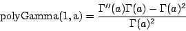 .
.
The syntax is:
| static double SpecialFunctions::polyGamma(int n,double a) |
n = 0 or 1 a > 0 |
We can try to model the stock market.
It usually follows a general procedure:
equilibrium-bubble-crash.
The stock prices will have this behavior:
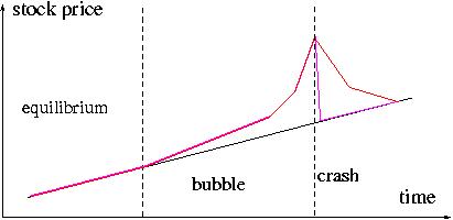
There are many possible crashes. A strong and short like the 1987 crash or a
"soft and long" one
like the Japanese crash of the nineties in Japan [Sautter1996].
However the result is similar, the stock prices returns to their "fundamentals".
In this section we are not interested in bubbles. For a very interesting
introduction and study of the properties of a bubble see [Sornette2004].
We can try to model this behavior with a kind of potential: think of a ball in
movement trapped in the following potential. The ball will move around the equilibrium.
The amplitude of the movement is the volatility.
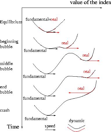
We are interested in the dynamics, i.e. how the ball moves in the potential.
However this dynamics will varies following the state of the market: equilibrium,
beginning-middle bubble-end bubble, crash and return to equilibrium.
Looks at the previous figure. If the market is in the "end bubble",
depending of the volatility (i.e. how the ball move around the local "real" equilibrium),
there is a probability not zero than the ball will "jump" to the
global equilibrium. This probability of jump does not exist in the period of equilibrium.
Therefore we must understand in which period we are to try to model
the dynamic of the stock market. Moreover it it specious to try to
get some general laws looking at the full history of the stock prices
without taking account of the different periods.
The usual procedure is to consider that the ball moves randomly
around the equilibrium. Moreover this random behavior will be
Normal
which is a very strong hypothesis which is surely wrong.
We will relax this hypothesis calculating an
implied volatility
from the market.
To be correct this procedure assumes that the market correctly prices the different
financial products present.
This could be true in equilibrium period but,
unfortunately, not true at the end of a bubble.
This section should be careful read. Indeed we will introduce some fundamental principle on option pricing which can be better understandable on this simple model.
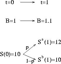
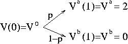
We can try to calculate the price of the option using our
estimated real probability preal=0.99 and discounting the result
with B(0)/B(1):
Vwrong(t=0) = (preal Va(1)
+ (1-preal) Vb) B(0)/B(1)
Vwrong(0) = (0.99 * 2 + 0.01 * 0) 1/1.1 = 1.98/1.1 = 1.8
Why it is wrong: arbitrage:
We construct a portfolio Π with a short option (i.e. be sell an option
that we do not have)
and a long stock (i.e. we buy the stock).
Π = -V + S
we have:
Π(0) = -V(0) + S(0) = -1.8 + 10 = +8.2
Πa(1) = -Va(1) + Sa(1) = -Va + Sa = -2 + 12 = + 10
Πb(1) = -Vb(1) + Sb(1) = -Vb + Sb = -0 + 10 = + 10
Therefore the portfolio Π gives the same result for the two possibilities
at time t=1: Π(1)=+10 and discounting it to compare it with Π(0):
Π(1).discount = Π(1) B(0)/B(1)= +10 * 1/1.1 ∼ +9.0909
We remark that Π(1).discount > Π(0)
which means that our portfolio increases its values for all
possibilities. So we can earn a lot of money … Unfortunately there is no
"free lunch", at least not so easy. So we conclude that
our value of V(0) is too big.
A correct answer: arbitrage:
The last paragraph gives the correct method to price the option: we
should not have arbitrage. We construct a portfolio with an Option
and Δ stocks:
Π = V + Δ S
Πa(1) = 2 + Δ 12
Πb(1) = 0 + Δ 10
Now we choose Δ such as Πa = Πb , i.e.
there is no more random component in the price of Π(1).
Δ = - (Va-Vb) / (Sa-Sb)
= - (2 -0)/(12-10) = -1
Then we have:
Π = V - S
Πa(1) = Πb(1) = -10
And since there should not be arbitrage we should have:
Π0 = Π(1).discount = Π(1) B(0)/B(1)
V(0) - S(0) = Π(1) B(0)/B(1)
V(0) = S(0) + Π(1) B(0)/B(1) = 10 - 10/1.1 = 1/1.1 ∼ 0.909
Which is almost two times smaller than our original guess 1.8.
We can now calculate the probabilities we must use to calculate
a correct answer. We must have :
V(0) = discount.(p Va + (1-p) Vb)
V(0) = B(0)/B(1).(p Va + (1-p) Vb)
p = (V(0) B(1)/B(0) - Vb)/(Va - Vb)
p = (1/1.1*1.1/1 - 0)/(2 - 0) = 1/2 = 0.5
We note that this probability is different from our estimate of
the "real" one p=0.99
First we calculate
the probability p using the fact the S/B is a martingale, i.e.
S(0)/B(0) = ∑ probability S(1)/B(1)
S(0)/B(0) = (p Sa + (1-p) Sb) / B(1)
This express the fact that the stock should grows at the same rate
as the interest rate to calculate the option. In
our example this read:
10/1 = (p 12 + (1-p) 10)/1.1
10*1.1 - 10 = p (12-10) = 2 p
p = 1/2 = 0.5
Second we calculate the option using this probability:
V(0)/B(0) = ∑ probability V(1)/B(1)
V(0)/B(0) = (p Va + (1-p) Vb) / B(1)
V(0)/1 = (0.5*2 + 0.5*0 ) / 1.1 = 1/1.1 ∼ 0.909
We obtain indeed a similar result than with the arbitrage
reasonning, in a much faster way.
To demonstrate why it works we will begin with the equation:
V(0)/B(0) = ∑ probability V(1)/B(1)
use the equation given by arbitrage considerations:
Π(0)/B(0) = Π(1)/B(1)
to prove that we obtain indeed:
S(0)/B(0) = ∑ probability S(1)/B(1)
We have
V(0)/B(0) = (p Va + (1-p) Vb) / B(1)
But from arbitrage considerations we know that choosing a correct value
of Δ we obtain that:
Π(0)/B(0) = Π(1)/B(1)
(V(0) + Δ S(0))/B(0) = (Va(1) + Δ Sa(1))/B(1)
(V(0) + Δ S(0))/B(0) = (Vb(1) + Δ Sa(1))/B(1)
Which can be rewritten as:
Va/B(1) = V(0)/B(0) + Δ S(0)/B(0) - Δ Sa/B(1)
Vb/B(1) = V(0)/B(0) + Δ S(0)/B(0) - Δ Sb/B(1)
Inserting these equations in the equation for V/B we obtain:
V(0)/B(0) = (p + (1-p)) V(0)/B(0) + Δ (p +(1-p)) S(0)/B(0)
- Δ (p Sa/B(1) + (1-p) Sb/B(1))
S(0)/B(0) = p Sa/B(1) + (1-p) Sb/B(1)
S(0)/B(0) = ∑ probability S(1)/B(1)
and we are done.
We take now 1/S as numeraire. The probability p' ≠ p.
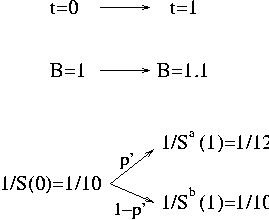
First we calculate
the probability p using the fact the B/S is a martingale, i.e.
B(0)/S(0) = ∑ probability' B(1)/S(1)
B(0)/S(0) = (p' 1/Sa + (1-p') 1/Sb) B(1)
For our example this read:
1/10 = (p' 1/12 + (1-p') 1/10)*1.1
1/11 - 1/10 = p' (1/12-1/10) = -2/(12*10) p'
p' = = 6/11
Second we calculate the option using this probability:
V(0)/S(0) = ∑ probability V(1)/S(1)
V(0)/S(0) = p' Va/Sa + (1-p') Vb/Sb
V(0)/10 = 6/11*2/12 + 5/11*0/10 = 10/11 ∼ 0.909
We obtain indeed a similar result than with the arbitrage
reasonning, in a much faster way.
We can follow a demonstration almost similar to the
previous section.
We will begin with the equation:
V(0)/S(0) = ∑ probability V(1)/S(1)
use the equation given by arbitrage considerations:
Π(0)/B(0) = Π(1)/B(1)
and the equation:
B(0)/S(0) = ∑ probability B(1)/S(1)
To obtain an equation 0=0.
We have
V(0)/S(0) = p' Va/Sa + (1-p') Vb/Sb
But from arbitrage considerations we know that choosing a correct value
of Δ we obtain that:
Π(0)/B(0) = Π(1)/B(1)
(V(0) + Δ S(0))/B(0) = (Va(1) + Δ Sa(1))/B(1)
(V(0) + Δ S(0))/B(0) = (Vb(1) + Δ Sa(1))/B(1)
Which can be rewritten as:
Va = V(0) B(1)/B(0) + Δ S(0) B(1)/B(0) - Δ Sa
Vb = V(0) B(1)/B(0) + Δ S(0) B(1)/B(0) - Δ Sb
Inserting these equations in the equation for V/S we obtain:
V(0)/S(0) = V(0)/B(0) (p' B(1)/Sa + (1-p') B(1)/Sb)
+Δ S(0)/B(0) (p' B(1)/Sa + (1-p') B(1)/Sb)
-Δ (p' + (1-p'))
Or using the equation
B(0)/S(0) = ∑ probability B(1)/S(1)
B(0)/S(0) = p' B(1)/Sa + (1-p') B(1)/Sb
We obtain:
V(0)/S(0) = V(0)/B(0) * B(0)/S(0) + Δ S(0)/B(0) * B(0)/S(0) -Δ
V(0)/S(0) = V(0)/S(0) +Δ - Δ
0 = 0
and we are done.
We have now another stock Q and we want to know the value of an option at time t=0 with a payoff at time t=1 first of (Q-20)+ and then (Q-S)+.
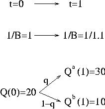
a. Calcul de q: Q/B is a martingale.
20/1 = q 30/1.1 + (1-q) 10/1.1
20*1.1 - 10 = q(30-10)
q = 12/20 = 0.6
b. Calcul of the option: V/B is a martingale. Payoff=(Q-20)+
V(0)/B(0) = q Va/B(1) + (1-q) Vb/B(1)
V(0)/1 = 0.6*10/1.1 + 0.4*0/1.1
V(0) = 6/1.1 ∼ 5.45
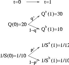
We know that since B/S is a martingale p'=6/11.
a. Calcul de q': Q/S is a martingale.
We consider now the four possibilities:
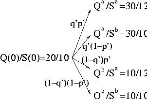
Q(0)/S(0) = q'p' Qa/Sa + q'(1-p') Qa/Sb
+ (1-q')p' Qb/Sa + (1-q')(1-p') Qb/Sb
= q' Qa (p'/Sa + (1-p')/Sb)
+ (1-q') Qb (p'/Sa + (1-p')/Sb)
= q' Qa/S(1) + (1-q') Qb/S(1)
with
1/S(1) = p'/Sa + (1-p')/Sb
1/S(1) = (p' B(1)/Sa + (1-p') B(1)/Sb)/B(1)
Or we have B/S is a martingale so:
B(0)/S(0) = p' B(1)/Sa + (1-p') B(1)/Sb
and we obtain:
1/S(1) = B(0)/(B(1)*S(0))=1/(1.1*10)=1/11
We can check it directly using the value of p' Sa and Sb:
1/S(1) = p'/Sa + (1-p')/Sb
1/S(1) = (6/11)/12 + (5/11)/10 = 120/(11*12*10) = 1/11
Therefore to calculate the probability q' we need to consider only two possibilities
with the numeraire 1/S:
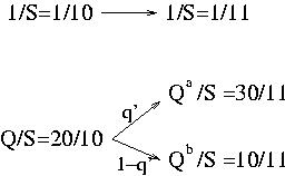
Q(0)/S(0) = q' Qa/S(1) + (1-q') Qb/S(1)
20/10 = q' 30/11 + (1-q') 10/11
2*11 - 10 = q' (30-10) = 20 q'
q' = 12/20 = 0.6 = q
It is normal that we found the same probability for Q in the two numeraires
(q for 1/B and q' for 1/S) because S/B is a martingale and therefore
S(0)/B(0)=S(1)/B(1) and the equations for q and q' are similar.
b. Calcul of the option: V/B is a martingale. Payoff=(Q-20)+
Since the payoff=(Q-20)+ does not depend of S we can use the
form:
1/S(0)=1/10 → 1/S(1)=1/11
and we have only two possibilities:
V(0)/S(0) = q' Va/S(1) + (1-q') Vb/S(1)
V(0)/10 = 0.6*10/11 + 0.4*0/11
V(0) = 6*10/11 ∼ 5.45
We find the same results. We will change now the payoff and
it will depend of S and Q.
The payoff at time t=1 is (Q-S)+.
a. 1/B as numeraire.
We have just seen that because Q/B and S/B are martingales
we obtain q=0.6 and
p=1/2.
To calculate the option we have to consider the martingale V/B for
the four cases:
V(0)/B(0) = (
qp (Qa-Sa)+
+ q(1-p) (Qa-Sb)+
+ (1-q)p (Qb-Sa)+
+ (1-q)(1-p) (Qb-Sb)+
)/B(1)
V(0)/1 = ( 0.6*0.5 (30-12)+ + 0.6*0.5 (30-10)+ + 0.4*0.5 (10-12)+ + r0=.4*0.5 (10-10)+ )/1.1
V(0) = (0.6*0.5*18 + 0.6*0.5*20)/1.1 = 11.4/1.1 ∼ 10.36
a. 1/S as numeraire.
We have just seen that because Q/S and B/S are martingales
we obtain q=0.6 and
p=6/11.
To calculate the option we have to consider the martingale V/S for
the four cases:
V(0)/S(0) =
q'p' (Qa-Sa)+/Sa
+ q'(1-p') (Qa-Sb)+/Sb
+ (1-q')p' (Qb-Sa)+/Sa
+ (1-q')(1-p') (Qb-Sb)+/Sb
V(0)/10 = 0.6*6/11*(30-12)+/12 + 0.6*5/11*(30-10)+/10
+ 0.4*6/11*(10-12)+/12 + 0.4*5/11*(10-10)+/10
V(0)/10 = 0.6*6/11*18/12 + 0.6*5/11*20/10 = 114/11 ∼ 10.36
This section was inspired by [Baxter1996], chapter 2.
We consider in this section several periods. We have this distribution
for the stock/Bond S/B:
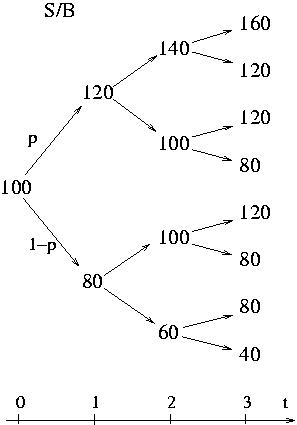
We take p=1/2. In this way S is a martingale with the numeraire B.
Indeed it is not difficult to check that at each node:
S(t-1)/B(t-1) = Average(S(t)/B(t))
We can define the filtration Fi as
the history of the stock up until the time i.
We have therefore
F0={100}
F1={100-120} or {100-80}
F2={100-120-140} or {100-120-100} or
{100-80-100} or {100-80-60}
F3={100-120-140-160} or {100-120-140-120} or {100-120-100-120} or {100-120-100-80}
{100-80-100-120} or {100-80-100-80} or {100-80-60-80} or {100-80-60-40}
And we can define the conditional expectation of X against filtration value i,
Ε(X(j) | Fi).
For this we sum X(j) for the paths defined by the filtration i.
We must have i ≤ j.
For example: S/B
| Expectation | Filtration | Value |
| Ε(S(3)/B(3) | F3) | {100-120-140-160} | 160 |
| Ε(S(3)/B(3) | F3) | {100-80-60-80} | 80 |
| Ε(S(3)/B(3) | F2) | {100-80-60} | 80/2 + 40/2 = 60 |
| Ε(S(3)/B(3) | F3) | {100-120-140} | 160/2 + 120/2 = 140 |
| Ε(S(3)/B(3) | F0) | {100} | 160/8+120/8+120/8+80/8+120/8+80/8+80/8+40/8=100 |
| Ε(S(2)/B(2) | F1) | {100-120} | 140/2+100/2=120 |
We note that whatever i and j we have:
S(i)/B(i) = Ε(S(j)/B(j) | Fi)
which is the definition of a martingale. Therefore we can say that under the mesure
Ρ corresponding to the probability {p,1-p}, S/B is a martingale.
An important theorem is the tower law:
Ε( Ε(X(k) | Fj) | Fi )
= Ε(X(k) | Fi)
with i ≤ j ≤ k
This is "obvious" but one example is always useful:
Ε( Ε(S(3)/B(3) | F2) | F0)
= Ε( (S(2)/B(2)=(160/2+120/2) or (120/2+80/2) or (120/2+80/2) or (80/2+40/2) following the path at time t=2) | F0)
= (160/2+120/2)/4 + (120/2+80/2)/4 + (120/2+80/2)/4 + (80/2+40/2)/4
= (160+120)/8 + (120+80)/8 + (120+80)/8 + (80+40)/8
= Ε(S(3)/B(3) | F0)
We have an option V(T)=(S/B-100)+ at time t=T=3. What is the value V(t)?
Using the fact that V should be a martingale with the numeraire B:
V(i)/B(i) = Ε(V(j)/B(j) | Fi)
it is not difficult to construct the corresponding tree. For example :
V(3)/B(3) = Ε(V(3)/B(3) | F3)
V(3)/B(3) =Ε(V(3)/B(3) | {100-120-140-160})= (160-100)+=60
V(3)/B(3) =Ε(V(3)/B(3) | {100-120-140-120})= (120-100)+=20
…
or
V(2)/B(2)= Ε(V(3)/B(3) | F2)
Can be written as
V(2)/B(2)= Ε(V(3)/B(3) | {100-120-140})=60/2+20/2=40
V(2)/B(2)= Ε(V(3)/B(3) | {100-120-100})=20/2+0/2=10
V(2)/B(2)= Ε(V(3)/B(3) | {100-80-100})=20/2+0/2=10
V(2)/B(2)= Ε(V(3)/B(3) | {100-80-60})=0/2+0/2=0
The resulting tree is:
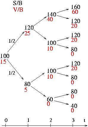
To calculate the option V(i) just multiply by B(i).
We can replicate our claim V just holding the right number of stocks and bonds.
Therefore it is not absolutely necessary to buy the derivative product.
However in case of jump of the stock price, for example during a crash, it
is possible that you cannot react fast enough to sell some stock. In this case
you could get a big loss.
Imagine that we have a portfolio Π and we hold φ stocks and ψ bonds.
We would like Π(t)=V(t) and that the portfolio is
self-financing, i.e. no need to add money.
First we need that
Π = V
φ(i) S(i) + ψ(i) B(i) = V(i)
φ(i) S(i)/B(i) + ψ(i) = V(i)/B(i)
Then at each node we need that our portfolio is self-financing. Imagine that
at time 0 we have φ(0) and ψ(0). Now we are at time 1, for example
for S(1)/B(1)=120. The value of Π(1)/B(1) is now:
Π(1)/B(1) = φ(0) S(1)/B(1) + ψ(0)
and we want to requilibrate the value of φ and ψ but do not add money.
We must therefore have:
Π(1)/B(1) = φ(1) S(1)/B(1) + ψ(1)
With these two equations and the fact that S and B are martingale we can prove
that
φ(i) = ΔV(i+1)/ΔS(i+1) = (ΔV(i+1)/B(i+1)) / (ΔS(i+1)/B(i+1))
ψ(i) = V(i)/B(i) - φ(i) S(i)/B(i)
With this choice we have Π=V:
Π(i) = φ(i) S(i) + ψ(i) B(i)
Π(i) = φ(i) S(i) + ( V(i)/B(i) - φ(i) S(i)/B(i) ) B(i)
Π(i) = V(i)
We can prove that the portfolio is self-financing but the best is surely to see
it on the example. In the next tree we have put the value of φ and ψ:
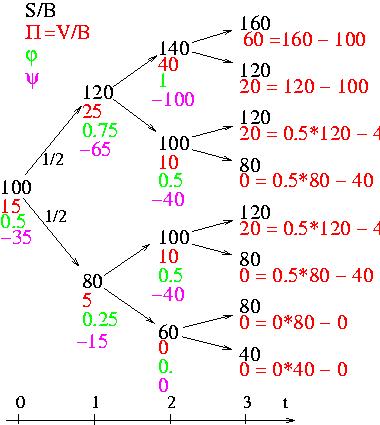
For example for the time t=1, S=120.
At time t=1- we have:
φ=φ(0) = 0.5
ψ=ψ(0) = -35
Π/B = 0.5*120 -35 = 25
At time t=1+ we have:
φ=φ(1) = 0.75
ψ=ψ(1) = -65
Π/B = 0.75*120 -65 = 25
And we can check that the relations are satisfied at each node. At time
t=T we do not update our portfolio and the value of:
Π(t=T=3)/B(3) = φ(2) * S(3)/B(3) + ψ(2)
gives the same result as the derivative V.
The calcul of the Hedge is similar to the prvious one for the replication
technic. If you sell the derivative (S/B-100)+, you can covert
your position holding a number φ of asset. For example in the previous
tree:
1. At time t=0 you sell your option for V(0)=15*B(0), i.e. you receive +15*B(0)
but you should think that the buyer of the option can exercice it, therefore
you should soustract -V(0)=-15*B(0) for your portfolio.
Moreover you borrow the money to buy
φ(0)=0.5 stock, i.e. you borrow
0.5 S(0)=50*B(0), therefore your portfolio at time
0 is therefore:
Π(0) = B(0)*(+15 - V(0) + φ S - 50) = 0
2. Now at time t=1, your portfolio is still equal to to 0.
First the money that you have borrowed from the bank, 50 B(0), and the money
that you have received, 15*B(0), if you have put the money
in a bank, must be multiply by B(1)/B(0). Therefore this part count as
+15*B(1) - 50*B(1)
If the new stock is equal to 120 your portfolio is:
Π(1)= +15*B(1) - 50*B(1) + 0.5*120*B(1) - V(1) = B(1)*(15 - 50 + 60 - 25) = 0
This is normal because φ(0) was chosen such as the random part due to the
stock price is canceled. However you should borrow some money and buy some
stock. Indeed imagine that you do nothing:
3.0 You have done nothing, i.e. you kept 0.5 stock, and the stock price jumps
to 140 at time t=2.
Π(2) = 15*B(2) - 50*B(2) + 0.5*140*B(2) - V(2) = B(2)*(15 - 50 + 70 - 40) = -5*B(2)
And if you keep this configuration untill the t=T you are no more covert.
3.1. At time t=1 you should borrow 0.25 S(1)=0.25*120*B(1)=30*B(1)
and buy 0.25 stock. Your portfolio at time t=1 is now still 0
Π(1)= B(1)*(V(0) - 0.5*S(0) -0.25*S(1) + 0.75*S(1)/B(1) - V(1)/B(1)) = B(1)*(15-50-30+90-25)=0
3.2. At time t=2, your portfolio is still equal to zero. As usual the money in the
bank must be multiplied by B(2)/B(1) and therefore if the stock is S(2)/B(2)=140:
Π(2)= B(2)*(V(0) - 0.5*S(0) -0.25*S(1) + 0.75*S(2)/B(2) - V(2)/B(2))
Π(2)= B(2)*(15-50-30+105-40)=0
3.3. We can check that if S(2)/B(2)=100 we obtain also 0:
Π(2)= B(2)*(15-50-30+75-10)=0
4.1. We continue until t=T=3. Take the case S(3)/B(3)=160.
Since S(2)/B(2)=160 > 100 the holder of the option will exercice it and we must
give a stock. But we have φ(2)=1 stock, therefore we do not need to buy any
stock. We will however receive 100, the strike of the option. Our
portfolio will be:
Π(3)= B(3)*(V(0) - 0.5*S(0) -0.25*S(1) -0.25*S(2) - 100)
Π(3)= B(3)*(15-50-30-35+100)=0
4.1. Imagine that we are in the path {100,120,100,120}. We have only
0.5 stock we must therefore buy 0.5 stock S(3) to deliver it to
the holder of the option. We will still receive 100, the strike of the option.
Our portfolio is therefore:
Π(3)= B(3)*(V(0) - 0.5*S(0) -0.25*S(1) +0.25*S(2) -0.5*S(3) + 100)
Π(3)= B(3)*(15 - 0.5*100 -0.25*120 +0.25*100 -0.5*120 + 100)
Π(3)= 0
You can check that all portfolio Π(3) gives 0. We are therefore
covert.
We consider the stock S and we write its behavior as
dS(0)/S(0)= (S(1)-S(0))/S(0) = 0.1 + 0.1 ε'
with ε'=&plusm; 1.
For S(0)=10 we obtain:
dS(0) = 1 + ε' and therefore S(1) = S(0) + dS(0) = 10 or 12 following
the sign of ε'.
We divide now our interval of time 1 in N steps dt:
N.dt=1 ⇒ N = 1/dt
and we want to found an expression for dS'/S' for the interval dt.
dS/S = Μ + Σ ε
After
N steps (at time t=1) we must have that the average of ε should be zeo
if N is big enough and there is no correlation between the ε. Therefore
we should have:
N Μ = 0.1
Μ = 0.1 /N = 0.1 * dt
Μ = μ * dt
After N steps the variance will add and we must have :
N Σ2 = 0.12
Σ = 0.1/N&fact12; = 0.1 dt&fact12;
Σ = σ dt½
Therefore we have:
dS/S = μ * dt + σ dt½ ε
At time t=1 after N steps we will have for one realisation:
dS/S = μ N dt + σ dt½ ∑0,N-1 ε
dS/S = μ + σ N-½ ∑0,N-1 ε
And the last term tends to a normal distribution of mean 0 and variance 1
following the central limit theorem.
dS/S = μ + σ Normal(0,1)
This holds as long as there is no correlations between the
random variables. This is surely wrong, but we hope not so much.
We introduce now the behavior of Stock prices. It will have a strong
resemblance with a Brownian motion where the particles do not interact
on each other but by the chocks between them. The point is that we can accept results
from this analyze while the hypothesis is valid. If it is not, great care must be
observed. In particular if we are in a bubble where the stock prices follow a kind
of phase transition [Sornette2004] the analyses based on this model could
be inexact.
We admit that the stock prices follow a Markov process, i.e. that the price at
t+1 is only determined by the price at t, or in other word all the past and
present information on a stock is included in the present price. This comes
from the assumption that the market is efficient. As explain in the previous
sections, this should work for a "standard" period but in a case of a bubble,
or of a crash, you should be aware that this assumption can break down.
Now we assume that the Stock price S follow a generalized Wiener process:
dS/S = μ dt + σ ε dt½
with μ is the drift rate per unit time, ε
is a random variable of a Normal distribution
of mean 0 and unit 1, and σ is the volatility of the stock (usually between
0.2 and 0.4).
We note that the second term cannot have an exponent α (for dtα)
different from 1/2. To understand this fact we consider a time
ΔT = N Δt with N → ∞ and Δt → 0.
The variance of S/S0
(i.e. of σεdtα) during Δt
is proportional to Δt2α. Therefore during the ΔT
the variance will be proportional to
N Δt2α=ΔT2α N1-2α.
This is valid
for any distribution of ε. If ε follow a Normal distribution
the variance is exactly equal to the sum of the variances. Otherwise, for another
distribution, there will exist a coefficient (2, or 4, or something, but constant,
and which should not depend of t). Then, if the theory is self consistent,
the variance of S should follow the same law for the variable t or T.
This imply that 1-2α=0 and therefore the exponent α=1/2.
If the volatility σ is 0 we have dS/S=μ dt ⇒ S = S0 eμt.
if σ ≠ 0
we can rewrite the equation as:
St = S0.Exp[ Normal ( (μ-σ2/2) t , σ t½ ) ]
S0 is the initial value.
Example:
We would like to know the price of a stock in 3 months = 1/4 year. We know that the volatility
per annum σ=30%, and the expected return (drift rate) μ=10%.
The current price of the action is S0=100$.
S1/4 = 100 Exp[ Normal((0.1-0.32/2)*0.5 , 0.3*(1/4)½) ]
or
S3 months = 100 Exp[ Normal(0.0275 , 0.15) ]
The principal problem in this analysis is that there is no reason
why the distribution should be normal and indeed it is not.
The point is that we know how to integrate exactly the integrals only in this
case and it is why in physics, for example, we impose this condition
and we calculate the corrections on this approximation.
In finance the procedure will not be to calculate the corrections but to
calculate an approximate σ. Obviously the procedure is a little bit silly:
we does not take the good distribution and then we try to "fix" it using
some tricks and in particular taken a σ which varies as function
of the some variables that we will introduce thereafter.
Everybody know the rule of three
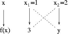
To calculate y we apply:
y * x1 = 3 * x2 ⇒ y = 3 * 2 / 1 = 6
This procedure is correct if f(x) = a*x.
Consider now a function
f(x) = x + a. The true result for f(x2) is 4 and not 6. Now
consider the same procedure for x3=1.01. With the rule
of three (f(x) = a*x) we obtain f(x3)=3.03 which is not "so far" from the
true result f(x3)=1.01+2=3.01.
Therefore the result will be as near as possible of the true result when:
We have in condensed our gold rules for option pricing.
First the function that we will
take to describe the variation of the stock price is a geometric Brownian one.
Even if it is far from perfect we hope that this function is not "too far"
from the real one.
Second we will calibrate the parameter of this function
(the volatility, the only parameter we can adjust)
using a reference not "too far", usually
the market price of a vanilla option.
Our procedure will fail if:
The class Options.hpp can calculate the value of an option
(call C or put P) using static functions, and calculate the value of Δ
the number of asset S that we need to hold to eliminate the randomness.
First we consider that the asset S does not pay out dividend.
Moreover we consider the vanilla option, i.e. the payoff at expiry t=T is
on the form max(S-E,0) for a call and max(E-S,0) for a put with E
the exercise price.
For the moment we consider that the interest rate r is constant
as the volatility σ of the asset S.
We know that dS can be written
as:
dS/S = μ dt + σ ε dt½
And we can apply the Ito's lemma for the option V(S,t)
with x=t, y=S, a=μ and b=σ:
dV(S,t) = ∂V/∂S σ ε dt½
+ (∂V/∂t + ∂V/∂S μ + ½ σ2 ∂2V/∂S2) dt + O(dt3/2)
We construct a portfolio Π with one option V and a number −Δ
of the underlying asset S:
Π = V -Δ.S
Using the previous equations for dS and dV, we arrive to:
dΠ = dV -Δ dS
dΠ = σ S (∂V/∂S - Δ) ε dt½
+ (μ S ∂V/∂S + ½ σ2 S2 ∂2V/∂S2
+ ∂V/∂t - μ Δ.S) dt
Choosing Δ=∂V/∂S we can eliminate the random component ε and the
portfolio is wholly deterministic:
dΠ =
( ½ σ2 S2 ∂2V/∂S2
+ ∂V/∂t) dt
Now we consider that the market are efficient and no arbitrage is possible, i.e.
that the risk free profit of invest money Π, rΠdt, should be equal to dΠ.
Using the definition of Π = V -Δ.S, we arrive to
the Black-Scholes equation:
∂V/∂t +
½ σ2 S2 ∂2V/∂S2
+ r S ∂V/∂S − r V = 0
with the conditions:
C(S,T)=max(S-E,0)
C(0,t)=0
C(S→∞,t) → S
for a call option, and for a put option:
P(S,T)=max(E-S,0)
P(0,t)=E e−r(T−t)
P(S→∞,t) → 0
We have this change of variables:
S = E ex ⇔ x = log(S/E)
t = T − τ/(σ2/2) ⇔ τ = (T−t) σ2/2
V = E v(x,τ) ⇔ v(x,τ) = V/E
Then we have:
∂/∂t = ∂τ/∂t ∂/∂τ = -σ2/2 ∂/∂τ
∂/∂S = ∂x/∂S ∂/∂x = 1/S ∂/∂x
∂2/∂S2 = − 1/S2 ∂/∂x
+ 1/S2 ∂2/∂x2
The Black-Scholes equation becomes:
∂v/∂τ = ∂2v/∂x2
+ (k−1) ∂v/∂x − kv with k=r/(σ2/2)
Now introducing:
v(x,τ) = eα x+ β τ u(x,τ)
∂v/∂τ = (β u + ∂u/∂τ) eα x+ β τ
∂v/∂x = (α u +∂u/∂x) eα x+ β τ
∂2v/∂x2 = (α2 u
+ 2 α ∂u/∂x + ∂2u/∂x2) eα x+ β τ
The equation reads:
∂u/∂τ = ∂2u/∂x2 + (2 α + k − 1) ∂u/∂x
+ (α2 + α (k−1) -k -β) u
Choosing:
2 α + k − 1 = 0 ⇔ α = −(k−1)/2
α2 + α (k−1) -k -β = 0 ⇔ β = −(k+1)2/4
We arrive to the equation of
diffusion:
∂u/∂τ = ∂2u/∂x2
With the variables:
V(S,t) = E v(x,τ) = E e− x (k−1)/2 −τ (k+1)2/4 u(x,τ)
V(S,t) = E(k+1)/2 S(k−1)/2 e(k+1)2(T-t) σ2/8 u( log(S/E) , (T-t) σ2/2 )
x = log(S/E)
τ = (T-t) σ2/2
k = r / (σ2/2)
There is two ways to solve it. The "standard"
way could be found in [Wilmott2000] for example.
The second way is to use Fourier transforms.
See [Kleinert] with a
theoretical physics formalism.
The result is:
u(x,τ) = 1/(4 π τ)½ ∫−∞+∞
u(y,τ=0) e−(x-y)2/4τ.dy
Or the condition on u(x,τ=0) (for a Call) can be written as:
u(x,τ=0) = V(S,T)/E e x (k−1)/2
u(x,τ=0) = max(S−E,0)/E e x (k−1)/2
u(x,τ=0) = max(ex−1,0) e x (k−1)/2
u(x,τ=0) = (e x−1) e x (k−1)/2 when x ≥ 0
u(x,τ=0) = (e x (k+1)/2−e x (k-1)/2) when x ≥ 0
Including it in the equation with the change of variable
x' = (y−x)/(2τ)½ we arrive to:
u(x,τ) = 1/(2π)½ ∫∞−x/(2τ)½
[ e((2τ)½ x'+x)(k+1)/2 −
e((2τ)½ x'+x)(k−1)/2
] e−x'2/2 dx'
Or we can use the relation:
(2τ)½ x'(k+1)/2 − x'2/2 =
− (x' − (2τ)½ x'(k+1)/2 )2 + τ (k+1)2/4
with the change of variable ρ=−(x' − (2τ)½ x'(k+1)/2),
to arrive to the equation:
u(x,τ) = e x (k+1)/2 + τ (k+1)2/4
1/(2π)½ ∫−∞(x+τ(k+1))/(2τ)½
e−ρ2/2dρ
- (k+1 → k−1)
The integral (with the 1/(2π)½ factor)
is the cumulative of the Normal distribution.
We are interested in the value of the option:
C(s,t) = E e− x (k−1)/2 - τ (k+1)2/4 u(x,τ)
C(s,t) = E e x FNormal((x+τ(k+1))/(2τ)½)
− E e−k τ FNormal((x +τ(k−1))/(2τ)½)
C(s,t) = S FNormal((x +τ(k+1)))/(2τ)½
- E e−r (T−t)
FNormal((x +τ(k−1)))/(2τ)½
Remembering that k=r/(σ2/2) and τ = (T−t) σ2/2,
the result can be written as :
C(S,t) = S FNormal(d1)
− E e−r(T−t)
FNormal(d2)
for a call option,and, for a put option:
P(S,t) = −S FNormal(−d1)
+ E e−r(T−t)
FNormal(−d2)
with
d1 = [ log(S/E) + (r + ½ σ2)(T−t) ]/ [σ (T−t)½]
d2 = [ log(S/E) + (r − ½ σ2)(T−t) ]/ [σ (T−t)½]
and FNormal is the cumulative of the Normal distribution. We note that these relations satisfy the Put-Call parity:
S + P − C = E e− r (T−t)
To demonstrate this formula we can think of a portfolio of one asset
S long, one call C short and one put P long.
The value at expiry t=T is E whatever the value of S.
The risk free present value
is therefore E e− r (T−t) and, from arbitrage
considerations, the two quantities should be equal.
Now if we want to define a portfolio Π composed of the option
and Δ assets S: Π = V - Δ S,
we must choose Δ=∂V/∂S to remove the randomness component:
ΔCall(S,t)=FNormal(d1)
ΔPut(S,t)=FNormal(d1)-1
The static functions available are:
| static double Options::European_Call (double S, double E, double T, double t, double r, double σ, double D0=0) |
| static double Options::European_Put (double S, double E, double T, double t, double r, double σ, double D0=0) |
| static double Options::Delta_European_Call (double S, double E, double T, double t, double r, double σ, double D0=0) |
| static double Options::Delta_European_Put (double S, double E, double T, double t, double r, double σ, double D0=0) |
|
Return the value of the call, put and delta |
It is interesting to plot the Options and Delta as function of S, E, and t
(the Δ for a put options can be found subtracting −1 to the
Δ for a call option):
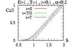
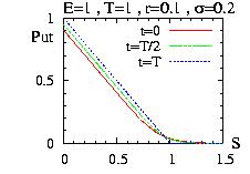
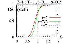
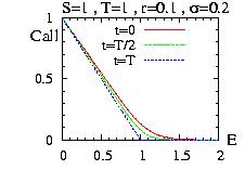
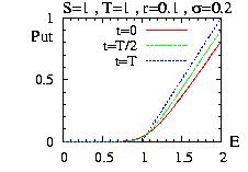
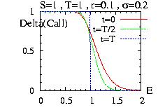
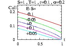
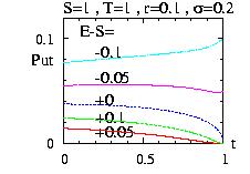
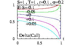
Example of program:
// Example Options_Vanilla1.cpp

#include "LOPOR.hpp"
using namespace LOPOR;

int main( )
{
    try
    {
        double E=1.;
        double S=1.;
        double r=0.1;
        double sigma=0.2;
        double T=1;
        double t=0;

        double Call=Options::European_Call(S,E,T,t,r,sigma);
        double Put=Options::European_Put(S,E,T,t,r,sigma);
        double D_Call=Options::Delta_European_Call(S,E,T,t,r,sigma);

        print("E=1, S=1, r=0.1, sigma=0.2, T=1; for t=0 we have:\n");
        print("Call(t=0)=",Call,", Put(t=0)=",Put);
        print("Delta_Call(t=0)=",D_Call,", Delta_Put=",D_Call-1.);

    }
    catch (const Error& error) { error.information( ); }
    return 0;
}
And the output is:
E=1, S=1, r=0.1, sigma=0.2, T=1; for t=0 we have:

Call(t=0)= 0.132697 , Put(t=0)= 0.0375342
Delta_Call(t=0)= 0.725747 , Delta_Put= -0.274253
The previous section treats the case where the payoff at time T is Λ(S)=max(S−E,0) for a call and Λ(S)=max(E−S,0) for a put. This section is concern with a general form of Λ.
The SOR method was introduced
to study partial differential equations. The reader should refer to the
corresponding section for more information
about the method.
The Method consist to give a solution at t=T, divide the time between t to T
in Nt, and for each time defined try to find a solution by iteration
using the Crank-Nicolson scheme. The static functions available are:
| static vector<double> Options::European (double payoff(const double& S), vector<double> boundaries(const std::vector<double>& Svector,const double& T_t), vector<double> S, int Nt, double T, double t, double r, double σ, double error_max=1.e-8, bool information=false) |
| static vector<double> Options::Delta_European (double payoff(const double& S), vector<double> boundaries(const std::vector<double>& Svector,const double& T_t), vector<double> S, int Nt, double T, double t, double r, double σ, double error_max=1.e-8, bool information=false) |
|
Return a vector of the value of the option and delta, for any
payoff function, and (option) the boundaries function,
at the updated vector S |
In the following example we calculate an European Put for E=10. We use two way. A direct using exact result, and a numerical one using the SOR method. We give the payoff(S)=max(E-S,0), and the boundaries: at S=Smin we have V(Smin,t)≈(E−Smin)*exp(r.(T-t)) and V(Smax,t)=0.
// Example European_SOR.cpp
// calcul an European Put P at t=0 with E=10
// using the SOR method and exact method

#include "LOPOR.hpp"
using namespace LOPOR;

double T=1, E=10, t=0.0 ;
double sigma=0.4, r=0.06;

double pay_off(const double& S)
{
    return Max(E-S,0.);
}

// boundaries: x=0 => E.exp(-r(T-t)); x=xmin => (E-xmin)*exp(-r(T-t))
// boundaries: x=oo => 0  ; x=xmax => 0
std::vector<double> boundaries(const std::vector<double>& S,const double& T_t)
{
    // return vector(boundary(xmin), boundary(xmax)
    return c2v((E-S[0])*exp(-r*T_t),0.);
}

int main( )
{
    try
    {
        std::vector<double> S0, S1, C0, C1;

        // using exact method:

        S0  =vec_create3(1.,21.,200);     // S={1,1.01,…,21}
        for(int i=0; i<S0.size(); ++i)
            C0.push_back(Options::European_Put(S0[i],E,T,t,r,sigma));

        // using the SOR method

        S1  =vec_create3(1.,21.,200);     // S1={1,1.01,…,21}
        int Nt=0;
        C1=Options::European(pay_off,boundaries,S1,Nt,T,t,r,sigma);

        // NOW S1 IS UPDATED:    S1={1,1.015,1.03,…,20.68,21}

        vec_print("European_SOR.res",S0,C0,S1,C1);
    }
    catch (const Error& error) { error.information( ); }
    return 0;
}
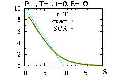
We can plot the third column (C0=exact) as function of the second column (S0),
and the fifth column (C1=SOR method) as function of the forth column (S1).
In the previous section the static functions available do a change of variable
x=log(S) and automatically update the vector S. However we are not forced
to do it and we can use the general formulation developped in
the section
Successive Over-Relaxation
for the general equation.
We begin by the equation for an option:
∂V/∂t +
½ σ2 S2 ∂2V/∂S2
+ r S ∂V/∂S − r V = 0
And we can use directly the static function
PartialDiffEqs::SOR.
Example of a program: We want to calculate an European Put option
with E=10, r=0.06, σ=0.3 at t=0 if the expiry date is T=1.
// Example SOR_European2.cpp
// equation
//
// dV/dt = a(x,t) d^2V/dx^2 + b(x,t) dV/dx + c(x,t) V + d(x,t)

#include "LOPOR.hpp"
using namespace LOPOR;

// payoff for a Put
double payoff(const double& x)
{
    double E=10.;
    return Max(E-x,0.);
}

int main( )
{
    try
    {
        double sigma=0.3, r=0.06, T=1;

        std::vector<double> S=vec_create3(0.,20.,20);

        // dV/dt = a(x,t) d^2V/dx^2 + b(x,t) dV/dx + c(x,t) V + d(x,t)
        // coeff={a,b,c,d}
        // a ={a(x0),a(x1),…}, b={…}, …
        std::vector<std::vector<double> >
            coeff(matrix_create<double>(4,S.size(),0.));
        for(int i=0; i<S.size(); ++i)
        {
            coeff[0][i]=power(sigma*S[i])/2.;  // sign: Option t -> -t
            coeff[1][i]=r*S[i];
            coeff[2][i]=-r;
            coeff[3][i]=0.;
        }

        // V(S,t=T)
        std::vector<double> V(S);
        for(int i=0; i<S.size(); ++i)
            V[i]=payoff(S[i]);

        double error_max=1.e-8;   // max error between two iterations (option)
        double w=1.1;    // Over relaxation (option)

        double dt=T/3.;
        int loops;

        // For t=2*T/3:
        V[0]=payoff(S[0])*exp(-r*(T-2*T/3));  // update the boundaries
        loops=PartialDiffEqs::SOR(S,dt,V,coeff,w,error_max);
        print("t=2T/3:  number of loops=  "+c2s(loops));

        // For t=T/3:
        V[0]=payoff(S[0])*exp(-r*(T-T/3));    // update the boundaries
        loops=PartialDiffEqs::SOR(S,dt,V,coeff,w);
        print("t=T/3:  number of loops=  "+c2s(loops));

        // For t=0:
        V[0]=payoff(S[0])*exp(-r*T);    // update the boundaries
        loops=PartialDiffEqs::SOR(S,dt,V,coeff);
        print("t=0:  number of loops=  "+c2s(loops));

        print("Results wrote in file \"SOR_European.res\": (i,S,Option)");
        vec_print("SOR_European.res",S,V);
    }
    catch (const Error& error) { error.information( ); }
    return 0;
}
And the output of the program is:
t=2T/3:  number of loops=  18
t=T/3:  number of loops=  20
t=0:  number of loops=  15
Results wrote in file "SOR_European.res": (i,S,Option)
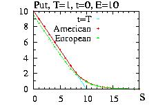
And we can plot the results using the file "SOR_European.res". We have also
plot the results for an American option calculated with the program
SOR_American2.cpp.
The Crank-Nicolson's method with LU decomposition was introduced
to study partial differential equations. The reader should refer to the
corresponding section for more information
about the method.
We show thereafter the program to calculate the European Vanilla Put
at t=0 for T=1, σ=0.2, E=10 and r=5%. We use the
relations:
∂u/∂τ = ∂2u/∂x2
V(S,t) = E v(x,τ) = E e− x (k−1)/2 −τ (k+1)2/4 u(x,τ)
V(S,t) = E(k+1)/2 S(k−1)/2 e(k+1)2(T-t) σ2/8 u( log(S/E) , (T-t) σ2/2 )
x = log(S/E)
τ = (T-t) σ2/2
k = r / (σ2/2)
to express the original value V(S,t) as function of U(x,τ), apply
the method, and then retrieve V(S,t). The program can be downloaded:
Put_Crank_Nicolson1.cpp
And the output is:
alpha= 0.752768 w= 1.05091
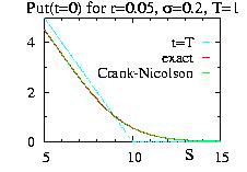
We can plot the result using the files "Put.res" for the exact result
(column 3 as function of column 2), and "res" for the numerical results
using the Crank-Nicolson's method (column 5 as function of column 4).
V(S,t) = e−r(T−t)
/ (2π(T−t)σ2)½
∫0∞ Λ(S')
e−(log(S'/S)−( r−σ2/2)(T−t) )2/2σ2(T−t) dS'/S'
V(S,t) =
∫0∞ Λ(S') P(S'/S)
It is interesting to plot the function P(S'/S) and v(S'/S)=Λ(S') P(S'/S):
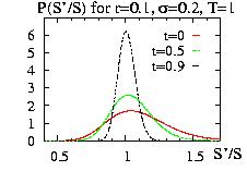
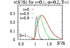
The function P(S'/S) is more centered around S'=S when t is nearer of T.
Moreover the integral increases when t approaches T.
This can be understood because this case corresponds to a constant payoff
equal to 1. In this case there is no risk and so the value of the option
is only the interest you can get putting it in the bank and get 1 after a time T,
i.e. e−r(T−t). We found indeed this result putting Λ(S')=1
in the formula above. In this case the value of the option increases as function of
the time.
The second
figure is plotted for the case Λ(S')=max(S'-E,0) with E=1. The integral
gives the value of the option. Only a small part of the integration space
contributes to the integral which is a perfect candidate for the
importance sampling procedure used by the Vegas method.
For this payoff the value of the integral (and the option)
decreases as function of the time.
This is due to the term (S-E)
for S>E which gives more importance to the queue of the
probabilities. However if you take another form for your payoff the option could decreases
as function of the time.
For example one exponential form centered around E.
The library provides one class to calculate the value of the option:
| static vector<double> Options::Binary (double payoff(const double& S),double S, double T, double t, double r, double σ,int MC=100000, int evaluation=1) |
|
Return a vector with the value of the option
calculated by Monte Carlo (Vegas) and the error = {value, error} |
Example of program:
// Example Binary.cpp
// calcul of the European Vanilla with Monte Carlo

#include "LOPOR.hpp"
using namespace LOPOR;

// Payoff
double E=1.0;
double payoff(const double& S)
{
    return MAX(S-E,0.);
}

int main( )
{
    try
    {
        std::vector<double> res;
        double S, T, t, r, sigma, exact;

        S=1.; T=1; t=0.5; r=0.1; sigma=0.2;
        res = Options::Binary(payoff,S,T,t,r,sigma);
        print("Call for S="+c2s(S)+", T="+c2s(T)+", r="+c2s(r)
                            +", sigma="+c2s(sigma)+", E="+c2s(E));
        print("By Monte Carlo (Vegas): I =",res[0],"+/-",res[1]);

        exact=Options::European_Call (S, E, T, t, r, sigma);
        print("Exact solution        : I =",exact);

    }
    catch (const Error& error) { error.information( ); }
    return 0;
}
And the output is:
Call for S=1, T=1, r=0.1, sigma=0.2, E=1
By Monte Carlo (Vegas): I = 0.082778 +/- 3.60035e-09
Exact solution        : I = 0.082778
The difference between the American and the European options is that
exercise is permitted at any time during the life of the options.
The consequence of it is that the value of an American
option cannot be less than the payoff. Indeed, if it was the case,
a risk free profit could be done. For example for a Put option
buying the corresponding asset
S and the option P, and exercise it immediately
selling the asset at the price E defined by the payoff.
Then the risk free profit will be −P−S+E which is positive
because P < E-S. In conclusion we have the condition:
V(S,t) ≥ payoff(S,E)
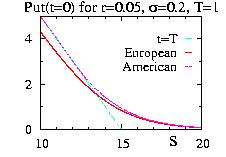
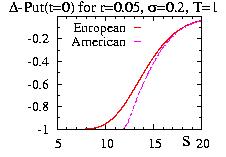
For example in the figure we have plotted the value of an European option and
an American option for E=15, T=1, t=0, r=0.05, σ=0.2 as function of
the value of the asset S. For S ≤ Sf
(Sf≈12 in the figures) the value of
the option P=payoff=max(E-S,0)=E-S.
For S > Sf the value of the option will reach
asymptotically the European value.
We can redo a similar analysis as the one we have done for the
derivation of the Black-Scholes equation for the European option.
We know that dS can be written
as:
dS/S = μ dt + σ ε dt½
And we can apply the Ito's lemma for the option V(S,t)
with x=t, y=S, a=μ and b=σ:
V(S,t) = ∂V/∂S σ ε dt½
+ (∂V/∂t + ∂V/∂S μ + ½ σ2 ∂2V/∂S2) dt + O(dt3/2)
We construct a portfolio Π with one option V and a number −Δ
of the underlying asset S:
Π = V -Δ.S
Using the previous equations for dS and dV, we arrive to:
dΠ = dV -Δ dS
dΠ = σ S /∂V/∂S - Δ) ε dt½
+ (μ S ∂V/∂S + ½ σ2 S2 ∂2V/∂S2
+ ∂V/∂t - μ Δ.S) dt
Choosing Δ=∂V/∂S we can eliminate the random component ε and the
portfolio is wholly deterministic:
dΠ =
( ½ σ2 S2 ∂2V/∂S2
+ ∂V/∂t) dt
The difference with the European option comes now.
We consider that the market are efficient and no arbitrage is possible, i.e.
that the risk free profit of invest money Π, rΠdt, should be
less or equal to dΠ. Indeed contrary to
the European option the American option can be exercised early.
Using the definition of Π = V -Δ.S, we arrive to
the Black-Scholes equation:
∂V/∂t +
½ σ2 S2 ∂2V/∂S2
+ r S ∂V/∂S − r V ≤ 0
For a Put this equation has these properties:
(∂u/∂τ − ∂2u/∂x2) . (u − g)=0
∂u/∂τ − ∂2u/∂x2 ≥ 0
u − g ≥ 0
with u(x→±∞,τ) = g(x,τ) and u(x,0) = g(x,0).
Unfortunately we cannot solve this problem, however we can apply numerical methods
and in particular the Successive Over-Relaxation (SOR)
method, slightly modified to take account of the condition u ≥ g.
The static functions available are:
| static vector<double> Options::American_Call (vector<double> S, double E, double T, double t, double r, double σ, double D0=0, double error_max=1.e-8, bool information=false) |
| static vector<double> Options::American_Put (vector<double> S, double E, double T, double t, double r, double σ, double D0=0, double error_max=1.e-8, bool information=false) |
| static vector<double> Options::Delta_American_Call (vector<double> S, double E, double T, double t, double r, double σ, double D0=0, double error_max=1.e-8, bool information=false) |
| static vector<double> Options::Delta_American_Put (vector<double> S, double E, double T, double t, double r, double σ, double D0=0, double error_max=1.e-8, bool information=false) |
|
Return a vector of the value of the call, put and delta,
at the updated vector S |
| static vector<double> Options::American (double payoff(const double& S), vector<double> boundaries(const std::vector<double>& Svector,const double& T_t), vector<double> S, int Nt, double T, double t, double r, double σ, double error_max=1.e-8, bool information=false) |
| static vector<double> Options::Delta_American (double payoff(const double& S), vector<double> boundaries(const std::vector<double>& Svector,const double& T_t), vector<double> S, int Nt, double T, double t, double r, double σ, double error_max=1.e-8, bool information=false) |
|
Return a vector of the value of the option and delta, for any
payoff function, and (option) the boundaries function,
at the updated vector S |
An example of program to calcul the Put option of an American Put with E=10., r=0.05, sigma=0.2, T=1. Calcul at t=0. (See also European_SOR_Put.cpp for an example of boundaries function)
// Example American_Put1.cpp
// E=10., r=0.05, sigma=0.2, T=1
// calcul an American Put at t=0
// using the projected SOR method

#include "LOPOR.hpp"
using namespace LOPOR;

double payoff_put(const double& S)
{
    return MAX(15.-S,0.);
}

int main( )
{
    try
    {
        double t=0, T=1., sigma=0.2, r=0.05;
        double E=15.;

        // create the vector S={1, 1.3, 1.6,…., 31} with 101 elements

        double Smin=1, Smax=31.;
        int    N=100;
        std::vector<double> S1, S2, S3, S=vec_create3(Smin,Smax,N);


        // !!! Since S is updated, save it for each call of an American function
        // however, if you do not change the value of Smin and Smax, S will not change

        std::vector<double> V=Options::American_Put(S,E,T,t,r,sigma);
        S1=S;

        // Now S={1, 1.03494,…, 29.9535, 31} : follows a log scale

        std::vector<double> Delta=Options::Delta_American_Put(S,E,T,t,r,sigma);
        S2=S;

        // using a payoff function
        // check that we get the same solution
        // information=true : some information about the functions are displayed
        // Nt=0 => the number Nt of time between T and t will be
        // automatically adjusted to obtain alpha=1

        int    Nt=0.;
        double D0=0.;
        bool information=true;
        double error_max=1.e-8;
        std::vector<double> V2=Options::American(payoff_put,S,Nt,T,t,r,sigma,D0,error_max,information);
        S3=S;

        vec_print("American_Put",S1,V,S2,Delta,S3,V2);

        // Comparison with European Vanilla put

        std::vector<double> delta, put, Svector;
        for(double s=Smin; s<= 5*E; s += 0.01)
        {
            Svector.push_back(s);
            put.push_back(Options::European_Put(s,E,T,t,r,sigma));
            delta.push_back(Options::Delta_European_Put(s,E,T,t,r,sigma));
        }
        vec_print("European_Put",Svector,put,delta);
    }
    catch (const Error& error) { error.information( ); }
    return 0;
}
And the output is:
alpha= 0.997663 w= 1.07152

tau=0.00117647, error less than 1e-08 in 5 loops
tau=0.00235294, error less than 1e-08 in 8 loops
tau=0.00352941, error less than 1e-08 in 9 loops
tau=0.00470588, error less than 1e-08 in 9 loops
tau=0.00588235, error less than 1e-08 in 10 loops
tau=0.00705882, error less than 1e-08 in 10 loops
tau=0.00823529, error less than 1e-08 in 10 loops
tau=0.00941176, error less than 1e-08 in 10 loops
tau=0.0105882, error less than 1e-08 in 10 loops
tau=0.0117647, error less than 1e-08 in 11 loops
tau=0.0129412, error less than 1e-08 in 11 loops
tau=0.0141176, error less than 1e-08 in 11 loops
tau=0.0152941, error less than 1e-08 in 11 loops
tau=0.0164706, error less than 1e-08 in 11 loops
tau=0.0176471, error less than 1e-08 in 11 loops
tau=0.0188235, error less than 1e-08 in 11 loops
tau=0.02, error less than 1e-08 in 11 loops
We have used the files "American_Put" and "European_Put"
to plot the figure above.
The American Call option is similar to the European if there is no dividend
because the European Call without dividend is always > payoff.
In the case of dividend please refer to
Continuous dividend for American Options.
In the previous section the static functions available do a change of variable
x=log(S) and automatically update the vector S. However we are not forced
to do it and we can use the general formulation developped in
the section
Successive Over-Relaxation
for the general equation.
We begin by the equation for an option:
∂V/∂t +
½ σ2 S2 ∂2V/∂S2
+ r S ∂V/∂S − r V = 0
And we can use directly the static function
PartialDiffEqs::SOR.
Example of a program: We want to calculate an American Put option
with E=10, r=0.06, σ=0.3 at t=0 if the expiry date is T=1.
// Example SOR_American2.cpp
// equation
//
// dV/dt = a(x,t) d^2V/dx^2 + b(x,t) dV/dx + c(x,t) V + d(x,t)

#include "LOPOR.hpp"
using namespace LOPOR;

// payoff for a Put
double payoff(const double& x)
{
    double E=10.;
    return Max(E-x,0.);
}

// condition for an American put: V > payoff
double condition(const double& x, const double& utemp)
{
    return Max(utemp,payoff(x));
}

int main( )
{
    try
    {
        double sigma=0.3, r=0.06, T=1;

        std::vector<double> S=vec_create3(0.,20.,20);

        // dV/dt = a(x,t) d^2V/dx^2 + b(x,t) dV/dx + c(x,t) V + d(x,t)
        // coeff={a,b,c,d}
        // a ={a(x0),a(x1),…}, b={…}, …
        std::vector<std::vector<double> >
            coeff(matrix_create<double>(4,S.size(),0.));
        for(int i=0; i<S.size(); ++i)
        {
            coeff[0][i]=power(sigma*S[i])/2.;  // sign: Option t -> -t
            coeff[1][i]=r*S[i];
            coeff[2][i]=-r;
            coeff[3][i]=0.;
        }

        // V(S,t=T)
        std::vector<double> V(S);
        for(int i=0; i<S.size(); ++i)
            V[i]=payoff(S[i]);

        double error_max=1.e-8;   // max error between two iterations (option)
        double w=1.1;    // Over relaxation (option)

        double dt=T/3.;
        int loops;

        // update boundaries: no need for an American Put,
        // For t=2*T/3:
        loops=PartialDiffEqs::SOR(S,dt,V,coeff,w,error_max,condition);
        print("t=2T/3:  number of loops=  "+c2s(loops));

        // For t=T/3:
        loops=PartialDiffEqs::SOR(S,dt,V,coeff,w,condition);
        print("t=T/3:  number of loops=  "+c2s(loops));

        // For t=0:
        loops=PartialDiffEqs::SOR(S,dt,V,coeff,condition);
        print("t=0:  number of loops=  "+c2s(loops));

        print("Results wrote in file \"SOR_American.res\": (i,S,Option)");
        vec_print("SOR_American.res",S,V);
    }
    catch (const Error& error) { error.information( ); }
    return 0;
}
And the output of the program is:
t=2T/3:  number of loops=  18
t=T/3:  number of loops=  20
t=0:  number of loops=  15
Results wrote in file "SOR_American.res": (i,S,Option)
And we can plot the results using the file "SOR_American.res". We have also
plot the results for an American option calculated with the program
SOR_European2.cpp.
If the interest rate or the volatility are not constant we must modify
slightly the formulae. We consider that we know how the r and σ
will vary in the future.
The Black-Scholes equation can be written as:
∂V/∂t +
½ σ(t)2 S2 ∂2V/∂S2
+ r(t) S ∂V/∂S − r(t) V = 0
Introducing the following variables:
s = S eα(t)
v = V eα(t)
τ = γ(t)
with
α(t)=∫tTr(t') dt'
γ(t)=∫tTσ2(t') dt'
the Black-Scholes equation becomes:
∂v/∂τ −
½ s2 ∂2v/∂s2
= 0 .
and the coefficient are independent of time. We can redo the procedure
to find the Black-Scholes but we can simply take the solution of
the Black-Scholes model replacing
r → 1/(T-t) ∫tT r(t') dt'
σ2 → 1/(T-t) ∫tT σ2(t') dt'
To calculate the integrals, if r(t) and σ2(t) are smooth enough you should use the
Romberg Integration method. Otherwise you should use the
Vegas Monte Carlo method.
The Black-Scholes equation is similar to the previous section, and the
American section:
∂V/∂t +
½ σ2 S2 ∂2V/∂S2
+ (r-D0) S ∂V/∂S − r V ≤ 0
with the conditions D0 ≤ r, V(S,t) > payoff. The equality holds
for one part of the S space (S > Sf for a Put and S < Sf
for a call) and does not hold for the other part where V=payoff. For a Call
without dividend V is always bigger than the payoff and then Sf→∞.
With a dividend Sf is finite.
Now we can do the change of variables
already done for the European option:
V(S,t) = E v(x,τ) = E e− x (k'−1)/2
−τ
(
(k'−1)2/4 + k
)
u(x,τ)
x = log(S/E)
τ = (T-t) σ2/2
k = r / (σ2/2)
k' = (r-D0) / (σ2/2)
to arrive to the equations (for a call for example):
∂u/∂τ = ∂2u/∂x2 if x ≤ xf(τ)
u(x,τ) = g(x,τ) for x > xf(τ)
with g(x,τ)= E-1 e+ x (k−1)/2 + τ
(
(k'−1)2/4 + k
)
payoff(S,t=T).
Then it is not difficult to apply the projected SOR method.
The static functions available are defined here.
In the following figures
we have plotted the results for American call and put, and the European counterparts.
The parameters are: t=0, T=1, sigma=0.8, r=0.25, D0=0.20 and E=10.
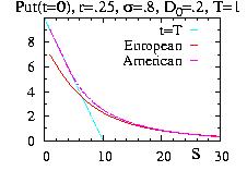
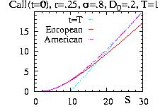
Admit that one dividend d.S will be paid at t=td between t=0 and t=T.
For td < t ≤ T no dividend is paid so the solution
is the normal Black-Scholes solution without dividend.
At t=td the dividend S.d is paid.
The value of the asset before and after td must be continuous
in time because the option does not receive the dividend. Otherwise an
arbitrager could make a risk-free profit.
V(S(td−),td−)=
V(S(td+),td+)
On the contrary the asset S must has a discontinuity in time because the owner
receive the dividend. From arbitrage consideration the asset S must
decrease by a value equal to the dividend:
S(td+)=S(td−)(1-d).
Therefore :
V(S,td−)=
V(S(1-d),td+)
// Example Discrete_Dividend.cpp
// calcul an European Call C at t=0 with E=10 and
// a discrete dividend a t=td of d.S

#include "LOPOR.hpp"
using namespace LOPOR;

double T=1, E=10, t=0.0, td=0.5, d=0.05;
double sigma=0.4, r=0.06;

double pay_off(const double& S)   // payoff at t=td for t≤td
{
    return Options::European_Call(S*(1.-d),E,T,td,r,sigma);
}

int main( )
{
    try
    {
        std::vector<double> S, C0, C1, C2, C3, C4;

        S   =vec_create3(1.,21.,200);     // S={1,1.01,…,20}

        for(int i=0; i<S.size(); ++i)
        {
            double p0, p1, p2, p3, p4;

            // without dividend at t=td-
            p0= Options::European_Call(S[i],E,T,td,r,sigma);

            // jump for the option t=td for t=td+
            p1= pay_off(S[i]);

            // result using numerical method at t=0
            p2= Options::Binomial(pay_off,S[i],20,td,t,r,sigma);

            // direct method at t=0
            p3= (1.-d)*Options::European_Call(S[i],E/(1.-d),T,t,r,sigma);

            // without dividend at t=0
            p4= Options::European_Call(S[i],E,T,t,r,sigma);

            C0.push_back(p0);
            C1.push_back(p1);
            C2.push_back(p2);
            C3.push_back(p3);
            C4.push_back(p4);
        }

        vec_print("Discrete_Dividend.res",S,C0,C1,C2,C3,C4);
    }
    catch (const Error& error) { error.information( ); }
    return 0;
}
European Call for T=1, E=10 and a discrete dividend at td=0.5
of d=0.05 S .
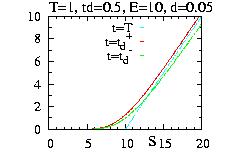
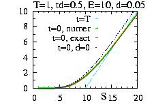
A compound option is an option on an option. We have an option C2 on an asset S at expiry date T2 and exercise price E2. Now we have another option C1 on the option C2 at expiry date T1 and exercise price E1. We have T2 ≥ T1 since there is no meaning to have an option on nothing if C2 is already out of date.
This is an example for an American or European Put option C1 on an American Put option C2:
// Example Compound.cpp
// calcul an European and an American Put C1 at t=0
// on an American Put C2 on option S.

#include "LOPOR.hpp"
using namespace LOPOR;


double T2=1  , E2=10;                  // option C2
double T1=0.5, E1=4, t=0;              // option C1
double sigma=0.4, r=0.06, D0=0.0;      // for the asset S: no dividend
int Nt=20;                             // for the Binomial method

double pay_off2(const double& S) {        // pay_off for the option C2 at time T2
    return Max(E2-S,0.);
}

double value_C2_T1(const double& S) {  // value of C2 at time T1
    return Options::Binomial(pay_off2,S,Nt,T2,T1,r,sigma,D0,"American");
}

double pay_off1(const double& S) {     // pay_off for the option C1 at time T1
     return Max(E1-value_C2_T1(S),0.);
}

double value_C1_t_Euro(const double& S) {   // value of C1 at time t
    return Options::Binomial(pay_off1,S,Nt,T1,t,r,sigma,D0,"European");
}

double value_C1_t_Amer(const double& S) {   // value of C1 at time t
    return Options::Binomial(pay_off1,S,Nt,T1,t,r,sigma,D0,"American");
}

int main( )
{
    try
    {
        std::vector<double> S, C2_T1, payoff_C1_T1, C1_t0_Euro, C1_t0_Amer;

        S            =vec_create3(0.,20.,200);     // S={0,0.1,…,20)
        C2_T1        =vec_func(value_C2_T1,S);     // C2 at t=T1
        payoff_C1_T1 =vec_func(pay_off1,S);        // =Max(E1-C2,0)
        C1_t0_Euro   =vec_func(value_C1_t_Euro,S); // C1 at t=0 for European option
        C1_t0_Amer   =vec_func(value_C1_t_Amer,S); // C1 at t=0 for American option

        vec_print("Compound.res",S,C2_T1,payoff_C1_T1,C1_t0_Euro,C1_t0_Amer);
    }
    catch (const Error& error) { error.information( ); }
    return 0;
}
And we have plotted the results in the following figures. Note: in the file
"Compound.res" the vec_print function writes
in the first column the number of the line. Therefore the second column
is S, the third is C2_T1, …
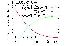
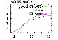
A chooser option is an option on an several options. For example we have two options: one put C2 and one call C3 on one asset S. The expiry dates are T2 and T3 and exercise prices E2 and E3. Now we have another option C1 and we have the choice to buy at time T1 the option C2 or the option C3. We have T2 ≥ T1 and T3 ≥ T1 since there is no meaning to have an option on nothing if C2 or C3 is already out of date.
This is an example for an European Call option C1 on an American Put option C2 and an American Call option C3:
// Example Chooser.cpp
// calcul an European Call C1 at t=0
// on an American  Put C2 or Call C3 on option S.

#include "LOPOR.hpp"
using namespace LOPOR;


double T2=1  , E2=10;                // option C2
double T3=1  , E3=10;                // option C3
double T1=0.5, E1=4, t=0;            // option C1
double sigma=0.4, r=0.06, D0=0.0;    // for the asset S: no dividend
int    Nt=20;                        // for the Binomial method

double pay_off2(const double& S) {    // pay_off for Put C2 at time T2
    return Max(E2-S,0.);
}

double pay_off3(const double& S) {    // pay_off for Call C3 at time T3
    return Max(S-E3,0.);
}

double value_C2_T1(const double& S) {  // value of C2 at time T1
    return Options::Binomial(pay_off2,S,Nt,T2,T1,r,sigma,D0,"American");
}

double value_C3_T1(const double& S) {  // value of C3 at time T1
    return Options::Binomial(pay_off3,S,Nt,T3,T1,r,sigma,D0,"American");
}

double pay_off1(const double& S) {     // pay_off for the option C1 at time T1
     return Max(value_C2_T1(S)-E1,value_C3_T1(S)-E1,0.);
}

double value_C1_t_Euro(const double& S) {   // value of C1 at time t
    return Options::Binomial(pay_off1,S,Nt,T1,t,r,sigma,D0,"European");
}

int main( )
{
    try
    {
        std::vector<double> S, C2_T1, C3_T1, payoff_C1_T1, C1_t0_Euro;

        S           =vec_create3(0.,20.,200);     // S={0,0.1,…,20)
        C2_T1       =vec_func(value_C2_T1,S);    // C2 at t=T1
        C3_T1       =vec_func(value_C3_T1,S);    // C3 at t=T1
        payoff_C1_T1=vec_func(pay_off1,S);        // =Max(C2-E1,C3-E1,0)
        C1_t0_Euro  =vec_func(value_C1_t_Euro,S); // C1 at t=0 for European option

        vec_print("Chooser.res",S,C2_T1,C3_T1,payoff_C1_T1,C1_t0_Euro);
    }
    catch (const Error& error) { error.information( ); }
    return 0;
}
And we have plotted the results in the following figures. Note: in the file
"Chooser.res" the vec_print function writes
in the first column the number of the line. Therefore the second column
is S, the third is C2_T1, …
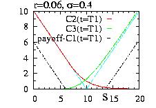
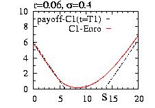
A barrier option with know-out is a normal option which becomes
worthless if the price of the asset S become lower (for a call: down-and-out)
than
the barrier value X, or more (for a put: up-and-out)
the barrier value X, at any time t.
This option is therefore path dependent.
We must not impose a upper barrier for a call or
a lower barrier for a Put. Indeed, imagine
that we impose for a call with a payoff(S,t)=max(S-E,t) a lower limit
X > E. We have at S ≤ X, and in particular at S=X:
Option=V(S=X,t)=0 for any t and in particular t=T-.
Or at t=T, V(S=X,T)=payoff(X,T)=X-E and the option
is not continuous in time.
Comparing to a normal option the change will simply be
that the boundaries conditions change: for a call
CNormal(S=0,t)=0 → COut(S=X,t)=0
And for a Put:
PNormal(S=∞,t)=0 → POut(S=X,t)=0
Numerically these conditions were indeed imposed choosing
the Smin and Smax in the section
about American options. Therefore there is no change for the
calculation of American option, at least using the SOR
method as in this previous section.
On the contrary the binomial method
cannot be applied directly in this case.
We will find now an exact formula for the European vanilla option.
As always the optimum conditions to calculate exactly a quantities
are at odd with the required conditions to do
numerical simulations. In the latter case we like discrete space,
with finite boundaries. In the former case we usually need
continuous space and infinite boundaries conditions.
In our case we have to find a way to reduce our problem with the boundaries
at S=X to a problem at ∞. Moreover it will be good if we
do not change the form of the equation to solve. The solution
is to use the method of images. It consists first to realize that the
diffusion equation:
∂u/∂t = ∂2u/∂x2
is invariant under a change of variable x→ −x and
x→x+x0, and so x→2x0 −x.
It is also invariant under the transformation u→ −u.
Moreover if u1 and u2 satisfy the same equation,
u1+u2 satisfies also the equation.
Therefore the way to implement the condition:
C(S=X,t)=0 ⇔ C(x=x0=log(X/E),τ)=0
is to consider the solution:
uOut=u(x,t) − u(2x0 − x,t)
For x=x0 we always have
uOut(x0,τ)=0 and since u(x,t)
and u(2x0 − x,t) satisfy the equation of diffusion,
their sum also satisfy it.
To find the formula for the option we have to use the relations:
V(S,t) = E v(x,τ) = E e− x (k−1)/2 −τ (k+1)2/4 u(x,τ)
V(S,t) = E(k+1)/2 S(k−1)/2 e(k+1)2(T-t) σ2/8 u( log(S/E) , (T-t) σ2/2 )
x = log(S/E)
τ = (T-t) σ2/2
k = r / (σ2/2)
to arrive to the equation:
VOut(S,t) = V(S,t) −
(S/X)−(k-1) V(X2/S,t) as X > S
VOut(S,t) = 0 as X ≤ S
And we have to consider only S ≥ X for a call, and S ≤ X for a Put. Example of program to construct the following figure:
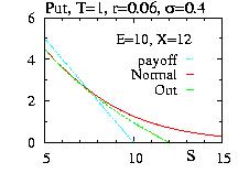
// Example Barrier2.cpp
// calcul an European Put P at t=0 with E=10 and
// a down-and-out form : if S>X => P=0

#include "LOPOR.hpp"
using namespace LOPOR;

int main( )
{
    try
    {
        double T=1, E=10, t=0;              // option P
        double sigma=0.4, r=0.06, D0=0.0, k=r/power(sigma); // for the asset S: no dividend
        double X=12;                         // The minimum barrier

        std::vector<double> S, P1, P_Barrier;

        S   =vec_create3(1.,21.,200);     // S={1,1.01,…,21}

        for(int i=0; i<S.size(); ++i)
        {
            double p1= Options::European_Put(S[i],E,T,t,r,sigma,D0);
            double p2= power(S[i]/X,-k+1)*Options::European_Put(X*X/S[i],E,T,t,r,sigma,D0);

            P1.push_back(p1);     // Normal Vanilla
            if(S[i]<X) P_Barrier.push_back(p1-p2);  // final result
            else       P_Barrier.push_back(0);      // final result
        }

        vec_print("Barrier2.res",S,P1,P_Barrier);
    }
    catch (const Error& error) { error.information( ); }
    return 0;
}
A barrier option with know-ins VIn is a normal option which is
worthless if the price of the asset S does not become
lower (for a call: down-and-in)
than
the barrier value X, or more (for a put: up-and-in)
the barrier value X, at any time t.
If the option reaches the limit at any time, it becomes a
normal option.
This option is therefore path dependent.
The best way to treat these option is to remark that:
VNormal(S,t) = VIn(S,t) + VOut
where VIn(S,t) is the option see in the
previous section and becomes useless
if the option cross the barrier X. Then we can find COut
using:
VIn(S,t) = VNormal(S,t) − VOut(S,t)
And for a vanilla option this reads:
VIn(S,t) =
(S/X)−(k-1) VNormal(X2/S,t) as X > S.
VIn(S,t) = VNormal(S,t) as X ≤ S
For an example of program see Barrier2.cpp.
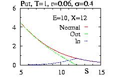
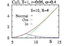
A lookback option is a derivative product whose payoff depends on the
maximum or minimum J realized asset price over the life of the option.
To apply Ito's lemma to an option V(S,J,t)
we need the variation
of J as function of dt. We First define Jn:
J = max(S(t)) = Jn→+∞
J = min(S(t)) = Jn→-∞
Jn = [
∫0t (S(τ))n.dτ
]1/n
We find:
dJn = dt.Sn.1/n.
[
∫0t (S(τ))n.dτ
]1/n - 1
dJn = dt.Sn/(n Jnn-1)
Jn is therefore a deterministic variable.
Applying Ito's lemma
we obtain for dV:
dV(S,J,t) = ∂V/∂S σ ε dt½
+ (∂V/∂t + ∂V/∂S μ + ½ σ2 ∂2V/∂S2 + Sn/(n Jnn-1) ∂V/∂Jn) dt + O(dt3/2)
We construct a portfolio Π with one option V and a number −Δ
of the underlying asset S:
Π = V -Δ.S
Using the previous equations for dS and dV, we arrive to:
dΠ = dV -Δ dS
dΠ = σ S (∂V/∂S - Δ) ε dt½
+ (μ S ∂V/∂S + ½ σ2 S2 ∂2V/∂S2 + Sn/(n Jnn-1) ∂V/∂Jn
+ ∂V/∂t - μ Δ.S) dt
Choosing Δ=∂V/∂S we can eliminate the random component ε and the
portfolio is wholly deterministic:
dΠ =
( ½ σ2 S2 ∂2V/∂S2 + Sn/(n Jnn-1) ∂V/∂Jn
+ ∂V/∂t) dt
Now we consider that the market are efficient and no arbitrage is possible, i.e.
that the risk free profit of invest money Π, rΠdt, should be equal to dΠ.
Using the definition of Π = V -Δ.S, we arrive to
the formula:
∂V/∂t +
½ σ2 S2 ∂2V/∂S2 + Sn/(n Jnn-1) ∂V/∂Jn
+ r S ∂V/∂S − r V = 0
n → ± ∞
The payoff for a lookback call is:
payoff(S,J) = max(S−J,0)
J=min(S(t)) for 0 ≤ t ≤ T
There exist an exact solution for this option:
C(S,J,t) = - S e−D0(T−t)[
-1 + (1 + 1/k) FNormal(-d7)
]
- J e−r(T−t)
[
FNormal(-d5)
− k−1 (S/J)1−k
FNormal(-d6)
]
with
d5 = [ log(J/S) − (r − D0 − ½ σ2)(T−t) ]/ [σ (T−t)½]
d6 = [ log(S/J) − (r − D0 − ½ σ2)(T−t) ]/ [σ (T−t)½]
d7 = [ log(S/J) + (r − D0 + ½ σ2)(T−t) ]/ [σ (T−t)½]
k = (r − D0)/(½ σ)
and FNormal is the cumulative of the Normal distribution. The static functions available are:
| static double Options::Lookback_European_Call (double S, double J, double T, double t, double r, double σ, double D0=0) |
|
Return the value of the put |
Example of program:
// Example Lookback_E_Call1.cpp

#include "LOPOR.hpp"
using namespace LOPOR;

int main( )
{
    try
    {
        double sigma=0.3, s2=sigma*sigma/2., r=0.06, T=1, t=0.;
        double J=10;

        // S={10,10.1,…,19.9,20}
        std::vector<double> S=vec_create3(J,20.,100);
        std::vector<double> Call(vec_create(S.size(),0.));
        std::vector<double> payoff(vec_create(S.size(),0.));

        for(int i=0; i<S.size(); ++i)
        {
            Call[i]= Options::Lookback_European_Call(S[i],J,T,t,r,sigma);
            payoff[i]= Max(S[i]-J,0.);
        }

        vec_print("lookback_E_call.res",S,Call,payoff);
    }
    catch (const Error& error) { error.information( ); }
    return 0;
}
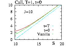
The European lookback call option with J=10.
You can also use the binomial model
or the MonteCarlo method.
The payoff for a lookback put is:
payoff(S,J) = max(J−S,0)
J=max(S(t)) for 0 ≤ t ≤ T
and we have always S ≤ J ⇒ Sn/(n Jnn-1) → 0 when n→±∞ and the differential equation
is the black-Scholes equation:
∂P/∂t +
½ σ2 S2 ∂2P/∂S2
+ r S ∂P/∂S − r P = 0
but with the conditions:
P(S,J,t) = max(J-S,0)
P(0,J,t) = J exp-r(T-t)
∂P/∂J (J,J,t) = 0.
The first condition is the payoff at expiry. The second comes from the
interest rate discounted at present of the payoff at expiry.
The last condition need a little bit more explanation.
Imagine that at time t the value of the asset S=J(t), i.e. the maximum
of the option so far. S follow a random walk and therefore
J(T) > J(t<T) with a probability 1.
But the option depend only of J(T) and therefore the option is insensitive of
small change around J(t).
There exist an exact solution for this option:
P(S,J,t) = S e−D0(T−t)[
-1 + (1 + 1/k) FNormal(d7)
]
+ J e−r(T−t)
[
FNormal(d5)
− k−1 (S/J)1−k
FNormal(d6)
]
with
d5 = [ log(J/S) − (r − D0 − ½ σ2)(T−t) ]/ [σ (T−t)½]
d6 = [ log(S/J) − (r − D0 − ½ σ2)(T−t) ]/ [σ (T−t)½]
d7 = [ log(S/J) + (r − D0 + ½ σ2)(T−t) ]/ [σ (T−t)½]
k = (r − D0)/(½ σ)
and FNormal is the cumulative of the Normal distribution. The static functions available are:
| static double Options::Lookback_European_Put (double S, double J, double T, double t, double r, double σ, double D0=0) |
|
Return the value of the put |
Example of program:
// Example Lookback_E_Put1.cpp

#include "LOPOR.hpp"
using namespace LOPOR;

int main( )
{
    try
    {
        double sigma=0.3, s2=sigma*sigma/2., r=0.06, T=1, t=0.;
        double J=10;

        // S={0,0.1,…,9.9,10}
        std::vector<double> S=vec_create3(0.,J,100);
        std::vector<double> Put(vec_create(S.size(),0.));
        std::vector<double> payoff(vec_create(S.size(),0.));

        for(int i=0; i<S.size(); ++i)
        {
            Put[i]= Options::Lookback_European_Put(S[i],J,T,t,r,sigma);
            payoff[i]= Max(J-S[i],0.);
        }

        vec_print("lookback_E_put.res",S,Put,payoff);
    }
    catch (const Error& error) { error.information( ); }
    return 0;
}
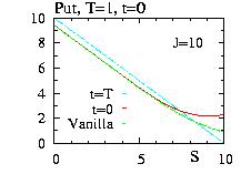
The European lookback put option with J=10.
You can also use the binomial model
or the MonteCarlo method.
An Asian option is a derivative product whose payoff depends on the
average asset price I realized over the life of the option.
To apply Ito's lemma to an option V(S,I,t)
we need the variation
of I as function of dt.
We First define I:
I = ∫0T f(S(τ),τ).dτ .
If f(S)=S we have the arithmetic average,
if f(S)=log(S) we have have the geometric average, but f can take
any form.
We have
dI = f(S,t).dt
and I is therefore a deterministic variable.
Applying Ito's lemma
we obtain for dV:
dV(S,I,t) = ∂V/∂S σ ε dt½
+ (∂V/∂t + ∂V/∂S μ + ½ σ2 ∂2V/∂S2 + f(S,t) ∂V/∂In) dt + O(dt3/2)
We construct a portfolio Π with one option V and a number −Δ
of the underlying asset S:
Π = V -Δ.S
Using the previous equations for dS and dV, we arrive to:
dΠ = dV -Δ dS
dΠ = σ S (∂V/∂S - Δ) ε dt½
+ (μ S ∂V/∂S + ½ σ2 S2 ∂2V/∂S2 + f(S,t) ∂V/∂I
+ ∂V/∂t - μ Δ.S) dt
Choosing Δ=∂V/∂S we can eliminate the random component ε and the
portfolio is wholly deterministic:
dΠ =
( ½ σ2 S2 ∂2V/∂S2 + f(S,t) ∂V/∂In
+ ∂V/∂t) dt
Now we consider that the market are efficient and no arbitrage is possible, i.e.
that the risk free profit of invest money Π, rΠdt, should be equal to dΠ.
Using the definition of Π = V -Δ.S, we arrive to
the formula:
∂V/∂t +
½ σ2 S2 ∂2V/∂S2 + f(S,t) ∂V/∂I
+ r S ∂V/∂S − r V = 0
We will consider the numerical solutions for the call arithmetic average f(S,t)=S.
The payoff for an average strike call option is:
payoff(S,t) = max(S − 1/t ∫0t S(τ) dτ , 0)
payoff(S,t) = S max(1 − 1/(S t) ∫0t S(τ) dτ , 0)
payoff(R,t) = S max(1 − R/t , 0)
R = 1/S ∫0t S(τ) dτ = I/S
With this form of payoff the option can be written as:
V(S,I,t) = S H(R,t)
and using this form we obtain the equation for H(R,t):
∂H/∂t +
½ σ2 R2 ∂2H/∂R2 +
∂H/∂R − r R ∂H/∂R = 0 .
We have used what s called a similarity reduction to reduce
the space of the problem from three (S,I,t) to two (R,t).
The conditions are:
H(R → +∞,t) = 0
∂H/∂t + ∂H/∂R = 0 when R → 0 and H must be finite
The first condition corresponds to R → +∞ ⇔ S→ 0 since
I is the average of S and therefore finite with a probability 1. Then
S << I and the option will not be exercised. The second
comes from a simplification of the differential equation.
The term R ∂R/∂R << ∂R/∂R for R→0.
The second term
R2 ∂2H/∂R2 is also negligible
near 0.
Indeed if H is finite near 0 we must have H=O(Rα)
with α > 0 and therefore
R2 ∂2H/∂R2 << ∂V/∂R.
With these condition and the differential equation we can use
the general method for partial differential equation
with Successive Over-Relaxation method.
We use this second formulation which correspond to our case. One example of program
can be found there:
Av_American2.cpp
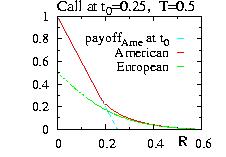
European and American options with
r=0.05, σ=0.8, T=0.5, at t0==0.25.
For an American option the differential equation becomes an inequality:
∂H/∂t +
½ σ2 R2 ∂2H/∂R2 +
∂H/∂R − r R ∂H/∂R ≤ 0 .
The solution is similar to the European case but with the condition H(R,t) ≥ payoff(R,t) (=Max(1-R/t,0) for a call). Using a linear complementary solution this condition is easily included using the general method for partial differential equation with Successive Over-Relaxation method. Example of program:
// Example Av_American2.cpp
// Calcul an European and American Call
// of an average strike option

#include "LOPOR.hpp"
using namespace LOPOR;

// payoff for a Put
double payoff(const double& x)
{
    return Max(1-x,0.);
}

double t;
// condition for an American put: V > payoff
double condition(const double& x, const double& utemp)
{
    return Max(utemp,payoff(x/t));
}

int main( )
{
    try
    {
        double sigma=0.8, r=0.05, T=0.5, t0=0.25;

        std::vector<double> R=vec_create3(0.,0.6,100);

        // dV/dt = a(x,t) d^2V/dx^2 + b(x,t) dV/dx + c(x,t) V + d(x,t)
        // dH/dt = -0.5*(sigma*R)^2 d^2H/dR^2 -(1-r R) dH/dR
        // coeff={a,b,c,d}
        // a ={a(x0),a(x1),…}, b={…}, …
        std::vector<std::vector<double> >
            coeff(matrix_create<double>(4,R.size(),0.));
        for(int i=0; i<R.size(); ++i)
        {
            coeff[0][i]=+power(sigma*R[i])/2.;  // sign: Option t -> -t
            coeff[1][i]=+(1.-r*R[i]);
            coeff[2][i]=0;
            coeff[3][i]=0.;
        }

        // V(R,t=T)
        t=T;
        std::vector<double> Ame(R), Eur(R);
        for(int i=0; i<R.size(); ++i)
        {
            Ame[i]=payoff(R[i]/t);
            Eur[i]=payoff(R[i]/t);
        }

        double dt=T/20.;
        int loops;

        for(t=T-dt; t>t0-ERROR; t-=dt)
        {
            loops=PartialDiffEqs::SOR2(R,dt,Ame,coeff,condition);
            print("t="+c2s(t)+":  American number of loops=  "+c2s(loops));
            loops=PartialDiffEqs::SOR2(R,dt,Eur,coeff);
            print("t="+c2s(t)+":  European number of loops=  "+c2s(loops));
        }

        print("Results wrote in file \"Av_American.res\": (i,R,Option)");
        print("Results wrote in file \"Av_European.res\": (i,R,Option)");
        vec_print("Av_American.res",R,Ame);
        vec_print("Av_European.res",R,Eur);
    }
    catch (const Error& error) { error.information( ); }
    return 0;
}
And the output is:
t=0.475:  American number of loops=  199
t=0.475:  European number of loops=  203
t=0.45:  American number of loops=  141
t=0.45:  European number of loops=  164
t=0.425:  American number of loops=  186
t=0.425:  European number of loops=  188
t=0.4:  American number of loops=  187
t=0.4:  European number of loops=  188
t=0.375:  American number of loops=  188
t=0.375:  European number of loops=  189
t=0.35:  American number of loops=  187
t=0.35:  European number of loops=  187
t=0.325:  American number of loops=  185
t=0.325:  European number of loops=  185
t=0.3:  American number of loops=  183
t=0.3:  European number of loops=  183
t=0.275:  American number of loops=  181
t=0.275:  European number of loops=  181
t=0.25:  American number of loops=  179
t=0.25:  European number of loops=  179
Results wrote in file "Av_American.res": (i,R,Option)
Results wrote in file "Av_European.res": (i,R,Option)
European and American options with
r=0.05, σ=0.8, T=0.5, at t0==0.25.
We define the geometric asset price average :
I = (Πi=1NSi)1/N
= exp( ∑i=1NSi / N)
and the payoff = max(I-E,0) for a call and max(E-I,0) for a put.
Since I is the product of lognormal distribution Si
it is also lognormally distributed. We can therefore obtain an exact formula. See
[Levy1997].
This chapter is very similar to the one for discrete dividend. We consider an arithmetic average strike option but any other function or other option type can be easily implemented.
We consider the model where I is not a
continuous average
of S but a discrete average:
I= ∑i=1N S(ti) .
There are N sampling date ti and the option depends
of the asset price S, the value of I, and the time t: V(S,I,t).
V(Si,Ii,ti+) = V(Si,Ii-1,ti-)
and we are able to calculate V(S,Ii-1,ti-).
The implementation of V(Si,Ii,ti+) =
V(Si,Ii-1,ti-) depends of the type
of the payoff. For a strike option it is:
payoffstrike(S,I,t)=max(S − I/t)
and so we have
V(S,I,t)=V(S+(Ii-Ii-1)/ti,Ii,t) if
ti-1+ < t ≤ ti
The arithmetic strike option is therefore easy enough to calculate, with
Ii-Ii-1=Si.
We introduce in this section the transaction cost. We will see that
they are fundamental for hedging a portfolio. We admit that the cost to sell
a share S is :
cost one share S = κ S .
Since the cost is not zero we cannot hedge our portfolio continuously, otherwise
the cost will explode. Therefore we are force to choose an interval of
time δt and hedge our portfolio every δt.
For example δ t=1 day=1/365 year.
We can now redo the development that we have done to find the
Black-Scholes equation but including
the transaction cost. In our portfolio we have Δ asset S and the
number of asset, ν, that we have to sell or buy to hedge our portfolio
is equal to the variation of Δ:
ν = Δ(S + δS, t + δt) -Δ(S,t)
ν = δS ∂Δ/∂S (S,t) + δt ∂Δ/∂t (S,t) + …
We know that
dS = μ S δt + σ ε S δt½
with μ is the drift rate per unit time, ε
is a random variable of a Normal distribution
of mean 0 and unit 1,
and for δt << 1 only the first term holds. We obtain with
Δ=∂V/∂S
ν = δS ∂Δ/∂S (S,t)
ν = ∂2V/∂S2 σ ε S δt½
Now the cost are always positive, whatever we hold the option long or short,
therefore the associate cost holding ν option is:
cost = |ν| κ S .
The average of |ε| is (2/π)½ and we obtain:
cost = (2/π)½ κ σ S2
|∂2V/∂S2| δt½ .
cost = (2/(πδt))½ κ σ S2
|∂2V/∂S2| δt .
We must soustract the cost of our portfolio for each transaction.
Therefore the Black-Scholes equation with transaction cost is:
∂V/∂t +
½ σ2 S2 ∂2V/∂S2
− (2/(π δt))½ κ σ S2
|∂2V/∂S2|
+ r S ∂V/∂S − r V = 0
This equation is nonlinear because of the presence of the absolute value. We note that from a numerical point of view the change is not so big as we will see it below.
Our portfolio has only one option held long. Moreover for a Vanilla European
option we have always ∂2V/∂S2 > 0.
Then the equation become a standard Black-Scholes equation with
a new σ'
σ'2 = σ2(1 − K)
K =(8/π)½ κ /(σ δ½)
For an option hold short, all sign must be inverse but the transaction cost
is still positive and we obtain:
σ'2 = σ2(1 + K)
There is therefore no problem to value an European option. This conclusion holds
for simple American option since we have
∂2V/∂S2 ≥ 0.
We have to minimize the risk (small δt) and the cost (large δt).
The best choice is to keep K around 1 or 0.5.
Example of program to calculate the value of an European put and the
corresponding Δ:
// Example Cost_European1.cpp
// European put option with cost kappa

#include "LOPOR.hpp"
using namespace LOPOR;

// payoff for a Put E=10.
double payoff(const double& x) { return Max(10.-x,0.); }

int main( )
{
    try
    {
        double sigma=0.4, r=0.06, T=1, kappa=0.01, E=10.;
        double t0=0.;
        double dt=T/400.;

        // S={0, 0.5, 1,…, 40}
        std::vector<double> S=vec_create3(0.,40.,80);
        std::vector<double> Put(S), Delta(S);

        // exact no cost:

        for(int i=0; i<S.size(); ++i)
        {
            Put[i]=Options::European_Put(S[i],E,T,t0,r,sigma);
            Delta[i]=Options::Delta_European_Put(S[i],E,T,t0,r,sigma);
        }

        vec_print("Exact_European.res",S,Put,Delta);
        print("Results wrote in file \"Exact_European.res\": (i,S,Option,Delta)");

        // exact with cost:

        double K=sqrt(8.)/sqrt(Pi*dt)*kappa/sigma;
        if(K>1) throw Error("K="+c2s(K)+" should be <1, increase dt");
        double sigmap=sigma*sqrt(1.-K);

        for(int i=0; i<S.size(); ++i)
        {
            Put[i]=Options::European_Put(S[i],E,T,t0,r,sigmap);
            Delta[i]=Options::Delta_European_Put(S[i],E,T,t0,r,sigmap);
        }

        vec_print("Exact_European_Cost.res",S,Put,Delta);
        print("Results wrote in file \"Exact_European_Cost.res\": (i,S,Option,Delta)");

    }
    catch (const Error& error) { error.information( ); }
    return 0;
}
The output of the program is:
Results wrote in file "Exact_European.res": (i,S,Option,Delta)
Results wrote in file "Exact_European_Cost.res": (i,S,Option,Delta)
The European Put and Delta for σ=0.4, r=0.06, T=1, κ=0.01, E=10.
The value of the option decreases if the cost is not zero.
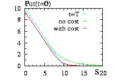
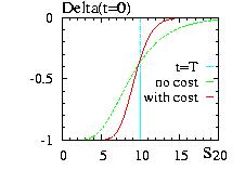
Our portfolio no longer has only one option held long
and therefore we do not have any more
∂2V/∂S2 > 0.
We can use the
explicit difference method
for this non linear equation:
∂V/∂t +
½ σ2 S2 ∂2V/∂S2
− (2/(π δt))½ κ σ S2
|∂2V/∂S2|
+ r S ∂V/∂S − r V = 0
Example of program to calculate the value of an European put and the
corresponding Δ:
The output of the program is:
// Example Explicit_Cost_European1.cpp
// European option with cost kappa
// Comparison with no cost
// Using Explicit Finite Difference

#include "LOPOR.hpp"
using namespace LOPOR;

// bullish vertical spread
double payoff(const double& x)
{
    double E1=8, E2=12;
    if(x<E1) return 0.;
    if(x<E2) return x-E1;
    return E2-E1;
}

int main( )
{
    try
    {
        double sigma=0.4, r=0.1, T=0.5, kappa=0.005;
        double t0=0.;
        double dt=T/400.;

        // calcul K
        double K=sqrt(8.)/sqrt(Pi*dt)*kappa/sigma;
        if(K>1) throw Error("K="+c2s(K)+" should be <1, increase dt");
        print("K=",K);

        // S={0, 0.5, 1,…, 40}
        std::vector<double> S=vec_create3(0.,40.,80);
        std::vector<double> Put(S), Delta(S);

        // no cost:

        for(int i=0; i<S.size(); ++i)
            Put[i]=Options::Binomial(payoff,S[i],100,T,t0,r,sigma);

        vec_print("European_noCost.res",S,Put,vec_derivative(Put,S));
        print("Results wrote in file \"European_noCost.res\": (i,S,Option,Delta)");

        // Explicit Finite difference with cost:

        // dV/dt = a(x,t) d^2V/dx^2 + b(x,t) dV/dx + c(x,t) V + d(x,t)
        //       +a'(x,t)|d^2V/dx^2|
        // coeff={a,b,c,d,a'},   a ={a(x0),a(x1),…}, b={…}, …

        std::vector<std::vector<double> >
            coeff(matrix_create<double>(5,S.size(),0.));

        for(int i=0; i<S.size(); ++i)
        {
            // sign: Option t -> -t
            coeff[0][i]=power(sigma*S[i])/2.;  // a
            coeff[1][i]=r*S[i];                // b
            coeff[2][i]=-r;                    // c
            coeff[3][i]=0;                     // d
            coeff[4][i]=-sqrt(2)/sqrt(Pi*dt)*kappa*sigma*power(S[i]); //a'
        }

        // Put(S,t=T):
        for(int i=0; i<S.size(); ++i)
            Put[i]=payoff(S[i]);

        for(double t=T-dt; t>-ERROR; t-=dt)
        {
            Put[S.size()-1]=payoff(S[S.size()-1])*exp(-r*(T-t));  // boundaries
            PartialDiffEqs::Explicit_Cost(S,dt,Put,coeff);
        }

        print("Results wrote in file \"Explicit_European_Cost.res\": (i,S,Option,Delta)");
        vec_print("Explicit_European_Cost.res",S,Put,vec_derivative(Put,S));

    }
    catch (const Error& error) { error.information( ); }
    return 0;
}
The output of the program is:
K= 0.56419
Results wrote in file "European_noCost.res": (i,S,Option,Delta)
Results wrote in file "Explicit_European_Cost.res": (i,S,Option,Delta)
The option and Delta for σ=0.4, r=0.1, T=0.5, κ=0.005, δt=0.5/400=0.00125 &assyp; half day.
The value of the option decreases if the cost is not zero.
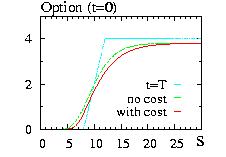
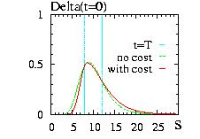
Imagine that the volatility σ is constant as function of the time.
To calculate it, we use the past data:
First we calcul the return
ri = Si/Si−1
and if we define the logarithm of the return:
ui = log(ri)
we can calculate the unbiased estimate of the volatility:
σ2 * dt =
∑i=1N( ui - average(u) )2 /(N − 1)
with dt the interval of time considered between ti
and ti+1.
Inside the class volatility we have define the static function
vol_unbiased to calculate the volatility:
| static double vol_unbiased(std::vector<double>& S, double& dt); |
|
Return the value of the unbiased volatility σ |
Example of a program:
// Example Volatility_Unbiased.cpp

#include "LOPOR.hpp"
using namespace LOPOR;

int main( )
{
    try
    {
        double S0=10;
        double r=0.25;
        double sigma=0.4;
        double dt=0.0001;
        double T=1.;

        // construction of the prices
        std::vector<double> S;
        S.push_back(S0);
        for(double t=0; t <=T; t += dt)
        {
            S0 *= exp((r-sigma*sigma/2.)*dt+sigma*sqrt(dt)*Normal::static_ran(););
            S.push_back(S0);
        }

        // Calcul of the unbiased volatility
        print("unbiased volatility=",Volatility::vol_unbiased(S,dt),", exact=",sigma);

    }
    catch (const Error& error) { error.information( ); }
    return 0;
}
And the result is:
unbiased volatility= 0.402177 , exact= 0.4
Unfortunately we cannot use this method because σ is not constant
Another method to obtain the volatility is to ascertain that the "market is right" which means that it is possible to get the volatility if we calculate which σ is necessary to get the the quoted price of options. Obviously if the market is wrong you get a wrong answer. We have implemented this function using the Broyden's method and the static function SolveEquations for a plain European Vanilla option.
| static double vol_implied(double& price,double& S,double& E, double& T, double& t, double& r, double& sigma, double& D0); |
|
Return the value of the unbiased volatility σ |
Example of a program:
// Example Volatility_Implied.cpp
// Calcul the implied volatility of IBM call option for
// Expiry= 4 months:  T=4/12
// Current price=S
// Dividend = D0
// Interest rate = r
// sigma_i = initial sigma for iteration
// Price = prices of the options as function of the Strike

#include "LOPOR.hpp"
using namespace LOPOR;

int main( )
{
    try
    {
        double S=63.92;
        double T=4./12.;
        double t=0;
        double r =0.0492;
        double D0=0.018;
        double sigma_i=0.6;

        // Price as function of the strike {35,40,…,155,160}
        std::vector<double> Strike=vec_create2<double>(35.,160.,5.);
        std::vector<double> Price;

        Price=c2v(30.5,25.3,20.5,16.80,12.6,9.3,6.4,4.1,2.60,1.5,0.9
                ,0.5,0.3,0.2,0.15,0.10,0.15,0.15,0.1,0.1,0.1
                ,0.1,0.1,0.05,0.05,0.05);

        // Calcul implied volatility
        std::vector<double> sigma;

        for(int i=0; i<Strike.size(); ++i)
        {
            sigma_i=Volatility::vol_implied(Price[i],S,Strike[i],T,t,r,sigma_i,D0,"Call");
            sigma.push_back(sigma_i);
        }

        // print in the file "Volatility1.res", the first line will be
        // "#E=   Price=   implied sigma="
        vec_print("Volatility_Implied.res",Strike,Price,sigma,"E=   Price=   implied sigma=");
    }
    catch (const Error& error) { error.information( ); }
    return 0;
The program create the file "Volatility_Implied.res":
#   i=         E=      Price=   implied sigma=
     0         35       30.5   0.900362
     1         40       25.3   0.692787
     2         45       20.5   0.575853
     3         50       16.8   0.587781
     4         55       12.6   0.510724
     5         60        9.3   0.484006
     6         65        6.4   0.450862
     7         70        4.1    0.42188
     8         75        2.6   0.411016
     9         80        1.5   0.394733
    10         85        0.9   0.392445
    11         90        0.5   0.385944
    12         95        0.3   0.388643
    13        100        0.2   0.398483
    14        105       0.15   0.414173
    15        110        0.1   0.420667
    16        115       0.15   0.476042
    17        120       0.15   0.504387
    18        125        0.1   0.502579
    19        130        0.1   0.527154
    20        135        0.1   0.550581
    21        140        0.1    0.57296
    22        145        0.1   0.594381
    23        150       0.05   0.567204
    24        155       0.05    0.58583
    25        160       0.05   0.603757
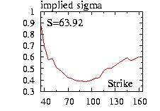
We can plot the implied volatility (column 4) as function
of the strike (column 2). We observe a "smile", the
volatility is not constant.
This is due to the fact that
the Black Scholes formula is not correct, and in particular
there is no reason why the random variation of the price dS/S
should be normal, i.e. that S will follow a lognormal distribution.
However there must exist also other reasons, for example some
correlations between the prices of the asset S as different
times. Therefore the "implied volatility" is a "clever" trick
to include the "corrections" to the Black Scholes equation.
One of the problem of this "clever" trick is that
if the market overprice or underprice
the real price, your result will have the same flaw.
Moreover the results will depend of the strike E but also of the
time to expiration T, at least. Indeed we could introduce several other
parameters. Moreover each option (American, Lookback, barrier, …)
will have a different implied volatility.
This is expected since the Black-Scholes theory does not integrate
the correct distribution nor the correlations, the corrections to include
will be different. In the next sections we will try to introduce some
models to try to avoid these pitfalls.
We can try to describe the variation of sigma using a non constant but known
parameter.
We note that this method cannot include the fact that the distribution
of ε is not normal.
1. σ(t) depends only of t. Then we can show
by a change of variable that nothing change if we consider
the new parameter γ :
γ=∫tTσ2(t') dt'
Therefore this method cannot explain the smile.
2. σ(S) depends only of S. Cox, Ross, and Rubinstein
[Cox1976,Cox1985] introduced
the constant elasticity of variance model using:
σ(S) = σ0 (S/S(0))γ-1
.
When γ < 0 the smile can be reproduce. However since there is only
one parameter and the model still continue to accept the normal distribution
as the correct one, it can reproduce only one smile (as function of the strike),
but not the smile,
or skew, as function of the time to expiry, or other variables.
3. σ(t,S) The two variables, S and t, are kept. With two parameters
we will be able to fit the entire surface for two parameters, for example
the Strike E and the expiry date T, for one option. But this calibration will
not work for another option. Brigo and
Mercurio [Brigo2001a,Brigo2001b]
have shown how to calibrate the model
Σ(t,S) to reproduce some surfaces.
dS/S = (r-D0) dt + σ ε dt½
The D0 is a constant dividend.
Now we are interested in the probability density function of S,
p(S,t; S',t').
We first apply the Ito's lemma for a function
f:
Δy = a Δx + b ε Δx½ .
df = ∂f/∂y b ε dx½
+ (∂f/∂x + ∂f/∂y a + ½ b2 ∂2f/∂y2) dx + O(dx3/2)
Considering y=S, x=t, a=(r-D0), b=σ, f(x,y)=f(t,S)=log(S) we obtain:
df = ((r-D0) − σ2/2) dt + σ ε dt½
i.e. df is normally distributed with mean ((r-D0) − σ2/2) dt and variance
σ2 dt. But f itself is the sum of all df (from t to t'),
and the sum of normal distributions is also a normal distribution,
with mean ((r-D0) − σ2/2) t and variance σ2 t.
At t we have f0=log(S), at t' we have f=log(S'),
the probability density function
is :
p(f) = e−(
f-f0−((r-D0) − σ2/2) t
)2/(2σ2t)
/(σ (2 π t)½ )
We want now get the probability distribution of S=ef. We have
P(f) df = P(S) dS/S and therefore.
p(S,t;S',t') = e−(
log(S'/S) − ((r-D0) − σ2/2) (t'-t)
)2/(2σ2(t'-t))
/(S σ (2 π (t'-t))½ )
With this probability we are able to calculate the average value
and the variance of S(t+δt) as function of S(t):
average = ∫0∞ S' p(S,t; S',t') dS'
average = e(r-D0) δt S(t)
variance = e2 (r-D0) + δt
(eσ2 δt − 1) S2
We note that the average can be calculated without the use of the
probability function. Indeed under the risk neutral argument
the average return of the asset S is exactly the one given by
the interest rate (r-D0) where the subtraction
is present because of the continuous dividend, i.e.
S(t) e(r-D0)δt. This argument
is also valid for an option but with
the rate r because the option receive no (continuous) dividend:
average(V(t+δt)) = V(t) erδt.
We will use this relation to calculate the option from the model we
introduce thereafter.
We will now construct a model which satisfied the equation for dS which is easy to manage numerically. First, we discretize the time between 0 and T in M: {0, δt, 2 δt, …, M δt=T}. Then we consider that an asset S at t could take two values:
We know that the value of S after
m steps is :
S(m,n) = dm−n un S0
where n is the number of time that the choice u was chosen (with a probability p),
and S0 is the price of the asset at t=0.
Moreover under the risk free concept
we have:
average(V(t+δt)) = V(t) erδt.
This formula read with (n+1) correspond to the choice of u,
n to the choice of d, m to the time t, and m+1 to t+δt:
p V(m+1,n+1) + (1-p) V(m+1,n) = V(m,n) erδt.
or equivalently:
V(m,n)=e−rδt ( p V(m+1,n+1) + (1-p) V(m+1,n) )
We are interested to calculate V(0,0), i.e. the value at the time t=0
(i.e. m=0) as function of the value of S0. We will do it
recursively. To calculate V(0,0) we need V(1,1) and V(1,0):
V(0,0)=e−rδt ( p V(1,1) + (1-p) V(1,0) )
Now to calculate V(1,1) we need V(2,1) and V(2,2), and to calculate
V(1,0) we need V(2,0) and V(2,1). We can continue the reasoning
to arrive that we have to know V(M,n) for n varying from 0 to M.
We know that for m=M, i.e. t=T, we have:
V(M,n)= payoff( S(M,n) )
with the payoff function equal to payoff(x)=max(E-x,0) for a put,
payoff(x)=max(x-E,0) for a call,
payoff(x)=Bθ(x-E) for a cash or nothing call, …
The
principle of the calculation will be:
| static double Options::Binomial (double payoff(const double& S),double S, int Nt, double T, double t, double r, double σ, double D0=0, string type="European", bool u_d=true) |
|
Return the value of the option. |
An example of program:
// Example Binomial_Options1.cpp with continuous dividend
// calcul an American Put at t=0
// E=10., T=1., sigma=0.3, r=0.06, D0=0.04, S=8.
// using Binomial method

#include "LOPOR.hpp"
using namespace LOPOR;


// Pay_off Put with E=10

double pay_off(const double& S)
{
    return Max(10.-S,0.);
}

int main( )
{
    try
    {
        double t=0, T=1., sigma=0.3, r=0.06, D0=0.04, S=8.;
        int Nt=50;
        std::string type="American";
        bool u_d;

        print("Binomial method:",type,", S=",S,", T=",T
                    ,", t=",t,", sigma=",sigma,", r=",r,", D0=",D0);

        u_d=false;
        print("(p=1/2): V=",Options::Binomial(pay_off,S,Nt,T,t,r,sigma,D0,type,u_d));

        u_d=true;
        print("(u=1/d): V=",Options::Binomial(pay_off,S,Nt,T,t,r,sigma,D0,type,u_d));

    }
    catch (const Error& error) { error.information( ); }
    return 0;
}
And the output of the program is
Binomial method: American , S= 8 , T= 1 , t= 0 , sigma= 0.3 , r= 0.06 , D0= 0.04
(p=1/2): V= 2.205
(u=1/d): V= 2.20843
For a path dependent option we cannot reconnect the tree as the
previous section for the non path dependent options. Therefore
we have to keep a memory of the path and construct a tree
of 2Nt possibilities, where Nt is the number of step (time).
The algorithm is therefore extremely simple:
Flaws of the algorithm:
Therefore for the option with the average of the asset price we will use this algorithm but for the lookback option (function of the minimum or maximum of the asset price) we will introduce another algorithm.
The arithmetic average J is defined as:
J=∑t=0N St / N
and the payoff could be any function of J and S, for example:
payoff(S,J)=max(S-J)
payoff(S,J)=max(E-J)
…
We have developped a static function:
| static double Options::Binomial_Arithmetic_Av (double payoff(const double& S, const double& J),double S, int Nt, double T, double t, double r, double σ, double D0=0, string type="European", bool u_d=true) |
|
Return the value of the option. |
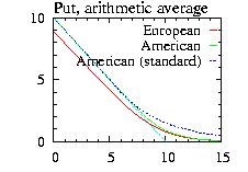
European and American Put for a arithmetic average option. For comparison
the result for a standard American option is displayed.
r=0.12, σ=0.5, no continuous dividend D0=0, 1 year at expiry, with
Nt=16 steps.
An example of program used to plot the figure:
// Example Binomial_Arithmetic_Av.cpp
// American Put with arithmetic average

#include "LOPOR.hpp"
using namespace LOPOR;

double pay_off(const double& S, const double& J)
{ return Max(10.-J, 0.); } // Arithmetic average

double pay_off2(const double& S)
{ return Max(10.-S, 0.); } // simple

int main( )
{
    try
    {
        int Nt=16;
        double T=1, t=0, r=0.12, sigma=0.5, D0=0.;

        std::vector<double> S=vec_create3(0.,20.,40);   // S={0, 0.5, 1, …, 20}
        std::vector<double> Eur=vec_create3(0.,0.,40);  // arithmetic average
        std::vector<double> Ame=vec_create3(0.,0.,40);  // arithmetic average
        std::vector<double> Am2=vec_create3(0.,0.,40);  // standard

        for(int i=0; i<S.size()-1; ++i)
        {
            Eur[i]=Options::Binomial_Arithmetic_Av(pay_off,S[i],Nt,T,t,r,sigma,D0,"European");
            Ame[i]=Options::Binomial_Arithmetic_Av(pay_off,S[i],Nt,T,t,r,sigma,D0,"American");
            Am2[i]=Options::Binomial(pay_off2,S[i],Nt,T,t,r,sigma,D0,"American");
        }

        print("Results wrote in file \"Binomial_Av1.res\": (i,S,Eur,Ame,Am2)");
        vec_print("Binomial_Av1.res",S,Eur,Ame,Am2);
    }
    catch (const Error& error) { error.information( ); }
    return 0;
}
And the output of the program is
Results wrote in file "Binomial_Av1.res": (i,S,Eur,Ame,Am2)
The arithmetic average J is defined as:
J=∑t=0N log(St) / N
and the payoff could be any function of J and S, for example:
payoff(S,J)=max(S-exp(J))
payoff(S,J)=max(E-exp(J))
…
We have developped a static function:
| static double Options::Binomial_Geometric_Av (double payoff(const double& S, const double& J),double S, int Nt, double T, double t, double r, double σ, double D0=0, string type="European", bool u_d=true) |
|
Return the value of the option. |
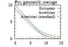
European and American Put for a geometric average option. For comparison
the result for a standard American option is displayed.
r=0.12, σ=0.5, no continuous dividend D0=0, 1 year at expiry, with
Nt=16 steps.
An example of program used to plot the figure:
// Example Binomial_Geometric_Av.cpp
// American Put with geometric average

#include "LOPOR.hpp"
using namespace LOPOR;

double pay_off(const double& S, const double& J)
{ return Max(10.-exp(J), 0.); } // geometric average

double pay_off2(const double& S)
{ return Max(10.-S, 0.); } // simple

int main( )
{
    try
    {
        int Nt=16;
        double T=1, t=0, r=0.12, sigma=0.5, D0=0.;

        std::vector<double> S=vec_create3(0.1,20.,40);   // S={0.1, …, 20}
        std::vector<double> Eur=vec_create3(0.,0.,40);  // geometric average
        std::vector<double> Ame=vec_create3(0.,0.,40);  // geometric average
        std::vector<double> Am2=vec_create3(0.,0.,40);  // standard

        for(int i=0; i<S.size()-1; ++i)
        {
            Eur[i]=Options::Binomial_Geometric_Av(pay_off,S[i],Nt,T,t,r,sigma,D0,"European");
            Ame[i]=Options::Binomial_Geometric_Av(pay_off,S[i],Nt,T,t,r,sigma,D0,"American");
            Am2[i]=Options::Binomial(pay_off2,S[i],Nt,T,t,r,sigma,D0,"American");
        }

        print("Results wrote in file \"Binomial_Av2.res\": (i,S,Eur,Ame,Am2)");
        vec_print("Binomial_Av2.res",S,Eur,Ame,Am2);
    }
    catch (const Error& error) { error.information( ); }
    return 0;
}
And the output of the program is
Results wrote in file "Binomial_Av2.res": (i,S,Eur,Ame,Am2)
The payoff for a lookback call is:
payoff(S,J) = max(S−J,0)
J=min(S(t)) for 0 ≤ t ≤ T
The payoff for a lookback put is:
payoff(S,J) = max(J−S,0)
J=max(S(t)) for 0 ≤ t ≤ T
There exist a solution for the European option for the call
and the put,
but not for an American option.
For the put option we
use the algorithm developped by [Babbs2000 ]. It consist
to consider instead of the variables S and J the variable N:
N(t) = log(J(t)/S(t))
And it can be proved that the only difference with a standard option
is a presence of a reflecting barrier in the tree (see article
for more information). Then the algorithm becomes very simple:
| static double Options::Binomial_Lookback_Put (double S, double J, int Nt, double T, double t, double r, double σ, double D0=0, string type="European") |
|
Return the value of the option. |
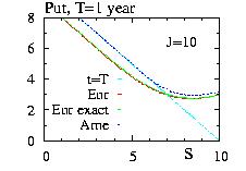
European and American Put for a lookback option with the binomial
approximation. For comparison
the result for a the exact results
for an European option is displayed.
r=0.1, σ=0.4, no continuous dividend D0=0, 1 year at expiry,
J=10, with Nt=1000 steps.
An example of program used to plot the figure:
// Example Binomial_Lookback_Put.cpp
// European and American Put Lookback option

#include "LOPOR.hpp"
using namespace LOPOR;

int main( )
{
    try
    {
        double T=0.5, t=0, J=10, r=0.1, sigma=0.2, D0=0.;
        int Nt=1000;

        // S={0,0.1,…,9.9,10}
        std::vector<double> S=vec_create3(0.,J,100);
        std::vector<double> Eur(vec_create(S.size(),0.));
        std::vector<double> Ame(vec_create(S.size(),0.));
        std::vector<double> Eur_exact(vec_create(S.size(),0.));

        for(int i=0; i<S.size(); ++i)
        {
            Eur[i]= Options::Binomial_Lookback_Put(S[i],J,Nt,T,t,r,sigma,D0,"European");
            Ame[i]= Options::Binomial_Lookback_Put(S[i],J,Nt,T,t,r,sigma,D0,"American");
            Eur_exact[i]= Options::Lookback_European_Put(S[i],J,T,t,r,sigma,D0);
        }

        vec_print("Binomial_Lookback_Put.res",S,Eur,Ame,Eur_exact);
        print("Results wrote in file \"Binomial_Lookback_Put.res\"");
    }
    catch (const Error& error) { error.information( ); }
    return 0;
}
And the output of the program is
Results wrote in file "Binomial_Lookback_Put.res"
We can reformulate (we follow [Clewlow1998])
the Binomial method to be able to choose an arbitrary large
time interval δt. We will not treat the asset price S but
the logarithm of S:
x = log(S)
We know that following Ito's lemma
and using a risk free concept
x follows the equation:
dx= (r − σ2/2) dt + σ ε dt½.
dx= ν dt + σ ε dt½.
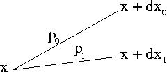
Therefore x can jump to x+δx0 with a probability p0=p, and
to x+δx1 with a probability p1=1−p.
p, δx0 and δx1
should give the correct answer for the average
and the variance of x:
average(dx) = ν dt = p δx0 + (1−p) δx1
average(dx2)
= σ2 δt + ν dt2
= p δx02 + (1−p) δx12
As before we have three unknown quantities
and two equations and we are free to choose one quantity:
p=1/2
δx0 = 0.5 ν δt
+ 0.5 (4 σ2 δt - 3 ν2 δt2)½
δx1 = 1.5 ν δt
- 0.5 (4 σ2 δt - 3 ν2 δt2)½
Or
p = 0.5 + 0.5 ν δt/δx0
δx0 = (σ2 δt + ν2 δt2)½
δx1 = - δx0
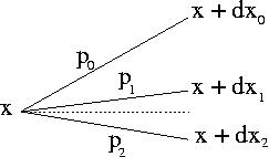
Using the formulation of the previous section (x=log(S)) we are able
to construct a trinomial tree (three branches instead of two).
We have
six unknown quantities (p0, p1, p2,
δx0, δx1, δx2)
and only three equations (for the average, the variance, and the sum of
probabilities is one):
ν δt = (r - σ2/2) δt
= p0 δx0
+ p1 δx1
+ p2 δx2
σ2 δt + ν2 δt2
= p0 + δx02
+ p1 + δx12
+ p2 + δx22
p0 + p1 + p2 =1
One of the solution is:
δx0 = δx2 = δx
δx1 = 0
p0 = (σ2 δt + ν2 δ2)/(2 δx2) + (ν δt)/(2 δx)
p0 = 1 - (σ2 δt + ν2 δ2)/(δx2)
p2 = (σ2 δt + ν2 δ2)/(2 δx2) - (ν δt)/(2 δx)
and we are free to choose δt and δx. We note that the trinomial tree
can be seen as an
explicit finite difference method.
The convergence criterion is:
δx > σ (3 δt)½
As we have seen, the volatility is not constant (see Volatility). We have
to take account of it when we construct the tree. One way is to construct
an "implied tree" [Derman1994,
Derman1995a,
Dupire1994]
(implied by the implied volatility) changing the value
of δx and δt at each step (x=log(S))
(see sections
Reformulation Binomial method
and Trinomial tree).
Consider the following tree with two steps:
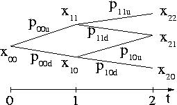
The jump "up",
dxiju=xi+1,j+1 - xi,j
and the jump "down",
dxijd=xi+1,j - xi,j
are all distinct for any i,j, and the probabilities are also different.
Also different are the
δti=ti+1-ti.
However we keep δti equal for all j.
We have for each point (i,j) a different volatility σij.
For the first step
we have four unknown quantities (σt, δx00u,
δx00d, p00u)
and two equations:
average(dx) = ν00 dt = p00u δx00u
+ p00d δx00d
average(dx2)
= σ002 δt0 + ν00 dt02
= p00u δx00u2
+ p00d δx00d2
with p00d = 1 - p00u and
ν00 = r - σ00
We are therefore free to choose δt and δx00u.
The next step require a little bit more care.
We have seven unknown quantities (σt,
δx10u, δx10d, p10u,
δx11u, δx11d, p11u)
and five equations:
(two for x10, see above)
(two for x11, see above)
x11+dx11d = x10+dx10u
We are therefore still free to choose δt and one other parameter.
We can generalize the procedure: the next step we will have 10 unknown
quantities and 8 equations, and so on. One way is to choose σt and
dxup=dxdown.
Now if we want to have more flexibility we can use a
Trinomial tree. It is not difficult to
implement this method. However as usual the binomial and trinomial tree
are restricted to one or two dimensions. For more we must use the
Monte Carlo methods.
In this section we consider the Monte Carlo method adapted to
the calcul of the options [Boyle1977].
For other applications see
the Monte Carlo section.
We will sometimes give the code i and not only some already made class.
In this way the reader can easily develop
his own code for other problems. However the code is
not optimized. For example we should
use the logarithm of the stock price S and not S to update S: it saves
a lot of exponential calls. However we hope that providing the most basic
code possible, the reader will grasp more clearly the main points
of the simulation.
We would like to calculate a
European Call Vanilla Option with
an exercise price E=10 for a current price S0=11 and
and expiry date T=1 year.
// Example MonteCarlo2.cpp
// European Call Vanilla option
// NOT OPTIMIZED

#include "LOPOR.hpp"
using namespace LOPOR;

double payoff(const double& S) { return Max(S-10.,0.); }

int main( )
{
    try
    {
        double T=1, t=0, r=0.1, sigma=0.2, D0=0.;

        int Nt=40;
        int NMC=10000;

        double S0=10.;
        double dt=(T-t)/c2d(Nt);

        double S, V, V2; // V= option, V2 for error

        V=0.; V2=0.;

        for(int iMC=0; iMC< NMC; ++iMC)
        {
            S=S0;
            for(int it=1; it<= Nt; ++it)
            {
                double epsilon=Normal::static_ran();
                S=S*exp((r-power(sigma)/2.)*dt+sigma*sqrt(dt)*epsilon);
            }
            V+=payoff(S);
            V2+=power(payoff(S));
        }
        V/=c2d(NMC);
        V2/=c2d(NMC);
        double error= sqrt((V2 - V*V)/c2d(NMC));

        // discount
        V *= exp(-r*(T-t));
        error *= exp(-r*(T-t));

        // result with Monte Carlo
        print("Monte Carlo           =",V,"+/-",error);

        // numerical integration
        std::vector<double> NI=Options::Binary(payoff,S0,T,t,r,sigma);
        print("numerical integration =",NI[0],"+/-",NI[1]);

        // exact
        double exact=Options::European_Call(S0,10,T,t,r,sigma);
        print("exact                 =",exact,"+/-",0.);
    }
    catch (const Error& error) { error.information( ); }
    return 0;
}
And the output is:
Monte Carlo           = 1.31795 +/- 0.0160593
numerical integration = 1.32697 +/- 8.38711e-07
exact                 = 1.32697 +/- 0
The two main flaws of the Monte Carlo simulations are:
We will see that there are some ways to reduce accelerate the simulations
and also to apply the monte Carlo to American options.
There are two main advantages of Monte Carlo simulations:
Importance sampling is very useful to make rare events less rare.
As shown there, the importance
sampling consists to simulate the random variable ε
with another distribution than the normal distribution of
zero mean. Obviously we have to include a factor to take
account of this choice. The procedure is:
Example of program to calculate a Vanilla European Call for E=10 and S0=7. Without importance sampling only a tiny fraction of the Monte Carlo obtain S(t=T) > E and therefore almost all give a zero contribution (something like 92%). Using a function g=Normal(mean=μ,variance=1) this rate decreases to 20%.
// Example MonteCarlo3.cpp
// Importance Sampling with g(x)=f(x=normal(mean=mu, variance=1))
// European Call Vanilla option
// NOT OPTIMIZED

#include "LOPOR.hpp"
using namespace LOPOR;

double payoff(const double& S) { return Max(S-10.,0.); }

int main( )
{
    try
    {
        double T=1, t=0, r=0.1, sigma=0.2, D0=0.;

        int Nt=40;
        int NMC=10000;
        double mu=0.35;

        double S0=7.;
        double dt=(T-t)/c2d(Nt);

        double S, V, V2, count; // V= option, V2 for error, % option != 0
        double S_IS, V_IS, V2_IS, count_IS; //  with importance sampling
        double factor;    // factor=f/g

        V=0.; V2=0.; count=0; V_IS=0.; V2_IS=0.; count_IS=0;

        for(int iMC=0; iMC< NMC; ++iMC)
        {
            S=S0;
            S_IS=S0;
            factor=1.;

            for(int it=1; it<= Nt; ++it)
            {
                double epsilon;

                // without importance sampling
                epsilon=Normal::static_ran();
                S=S*exp((r-power(sigma)/2.)*dt+sigma*sqrt(dt)*epsilon);

                // with importance sampling
                epsilon=Normal::static_ran(mu,1);
                factor *= Normal::static_density(epsilon)/Normal::static_density(epsilon,mu);
                S_IS=S_IS*exp((r-power(sigma)/2.)*dt+sigma*sqrt(dt)*epsilon);
            }

            V+=payoff(S);   // without importance sampling
            V2+=power(payoff(S));
            if(payoff(S)>0.) ++count;  // % success

            V_IS+=payoff(S_IS)*factor;   // with importance sampling
            V2_IS+=power(payoff(S_IS)*factor);
            if(payoff(S_IS)>0.) ++count_IS; // % success
        }

        // without importance sampling
        V /= c2d(NMC); V2 /= c2d(NMC);
        double error= sqrt((V2 - V*V)/c2d(NMC));
        V *= exp(-r*(T-t));  //discount
        error *= exp(-r*(T-t));  //discount
        count /= c2d(NMC);

        // with importance sampling
        V_IS /= c2d(NMC); V2_IS /= c2d(NMC);
        double error_IS = sqrt((V2_IS  - V_IS *V_IS )/c2d(NMC));
        V_IS  *= exp(-r*(T-t));  //discount
        error_IS  *= exp(-r*(T-t));  //discount
        count_IS /= c2d(NMC);

        // result with Monte Carlo
        print("Without importance sampling=",V,"+/-",error,", success=",count,"%");
        print("With    importance sampling=",V_IS,"+/-",error_IS,", success=",count_IS,"%");

        // numerical integration
        std::vector<double> NI=Options::Binary(payoff,S0,T,t,r,sigma);
        print("numerical integration      =",NI[0],"+/-",NI[1]);

        // exact
        double exact=Options::European_Call(S0,10,T,t,r,sigma);
        print("exact                      =",exact,"+/-",0.);
    }
    catch (const Error& error) { error.information( ); }
    return 0;
}
And the output is:
Without importance sampling= 0.0777977 +/- 0.00351103 , success= 0.0854 %
With    importance sampling= 0.0748292 +/- 0.000615031 , success= 0.7946 %
numerical integration      = 0.0748091 +/- 1.31142e-07
exact                      = 0.074809 +/- 0
We observe that the error has been divided by a factor 6 from 0.00351103 to 0.000615031.
Some more complicated case like a down-and-in barrier call option could even
lead to a more important gain [Boyle1997]. For other applications
see [Schoenmakers1997,Newton1997,Glasserman1999,Glasserman2004].
The control variate techniques use the knowledge of an exact solution G
which is not "too far" from the solution. It consists to
to calculate at the same time the estimate of the option f and the estimate
of the exact solution g. Then the estimate of the option using the control
variable technique is:
Option (control variate) = G + <f − g>
We give an example of program to calculate an European lookback put
option using as control variate the European put option:
// Example MonteCarlo4.cpp
// Lookback European Put
// with Control Variate (as Vanilla European Put)
// _CV= Control Variate
// NOT OPTIMIZED

#include "LOPOR.hpp"
using namespace LOPOR;

double J;
double Jini=10;
double payoff(const double& S) { return Max(J-S,0.); }
double payoff_CV(const double& S) { return Max(Jini-S,0.); }

int main( )
{
    try
    {
        double T=1., t0=0, r=0.06, sigma=0.3, D0=0.;

        int Nt=50000;   // large to get a precise  J=max(S)
        int NMC=10000;
        double S0=6.;
        double dt=(T-t0)/c2d(Nt);

        double S, V, V2; // V= option, V2 for error
        double    V_CV, V2_CV; //  control variate
        double G;  // result control variate
        G=Options::European_Put(S0,Jini,T,t0,r,sigma);
        double discount=exp(-r*(T-t0));

        V=0.; V2=0.; V_CV=0.; V2_CV=0.;

        for(int iMC=0; iMC< NMC; ++iMC)
        {
            S=S0;
            J=Jini;

            for(int it=1; it<= Nt; ++it)
            {
                double epsilon=Normal::static_ran();
                S=S*exp((r-power(sigma)/2.)*dt+sigma*sqrt(dt)*epsilon);
                J = Max(J,S);
            }

            double f = discount*payoff(S);     // normal
            double g = discount*payoff_CV(S);  // control variate

            V  += f;   // without control variate
            V2 += power(f);

            V_CV  += G + (f-g);   // control variate
            V2_CV += power(G + (f-g));
        }

        // without control variate
        V /= c2d(NMC); V2 /= c2d(NMC);
        double error= sqrt((V2 - V*V)/c2d(NMC));

        // with control variate
        V_CV /= c2d(NMC); V2_CV /= c2d(NMC);
        double error_CV = sqrt(fabs(V2_CV  - V_CV *V_CV )/c2d(NMC));

        // result with Monte Carlo
        print("Without control variate =",V,"+/-",error);
        print("With    control variate =",V_CV,"+/-",error_CV);

        // exact
        double exact=Options::Lookback_European_Put(S0,Jini,T,t0,r,sigma);
        print("exact                   =",exact,"+/-",0.);

        // binomial method
        double binomial=Options::Binomial_Lookback_Put(S0,Jini,10000,T,t0,r,sigma);
        print("Binomial                =",binomial,"+/- ?");

        // European put option
        double eur=Options::European_Put(S0,Jini,T,t0,r,sigma);
        print("European                =",eur,"+/-",0.);

    }
    catch (const Error& error) { error.information( ); }
    return 0;
}
And the results are:
Without control variate = 3.55523 +/- 0.0157347
With    control variate = 3.54604 +/- 0.00271254
exact                   = 3.54561 +/- 0
Binomial                = 3.53857 +/- ?
European                = 3.48279 +/- 0
The error are reduced by a factor 7 which means that we need 50 times (50 = 72 + …, errors follows a law NbMC−½) less time to obtain the same result as without control variate.
In this section we will try to have a "better" implementation of the normal distribution. There are several related methods: Latin Hypercubic method, antithetic variates, moment matching, quasi random sequences. All the methods try to correct the errors due to the randomness nature of the Monte Carlo using a special sampling of the normal distribution.
The method impose that the average of the random number from a normal distribution is zero. It is based on the fact that the Normal distribution is symmetric around 0 and therefore if the sequence {rani}, with i=0 to n follow a Normal distribution, then the sequence {-rani} should follow also a Normal distribution. Then we can average the two results from the two sequences. Example of program to calculate an European Vanilla Call and compare different methods:
// Example MonteCarlo5.cpp
// European Call Vanilla option
// _AV = Antithetic variables
// NOT OPTIMIZED

#include "LOPOR.hpp"
using namespace LOPOR;

double payoff(const double& S) { return Max(S-10.,0.); }

int main( )
{
    try
    {
        double T=1, t=0, r=0.1, sigma=0.2, D0=0.;
        double S0=10.;
        int    Nt=40;
        int    NMC=10000;

        double dt=(T-t)/c2d(Nt);
        double discount=exp(-r*(T-t));

        double S1, S2, V, V2, V_AV, V2_AV; // V= option, V2 for error

        V=0.; V2=0.;
        V_AV=0.; V2_AV=0.;

        // Monte Carlo
        for(int iMC=0; iMC< NMC; ++iMC)
        {
            S1=S0;
            S2=S0;
            for(int it=1; it<= Nt; ++it)
            {
                double epsilon=Normal::static_ran();;
                S1=S1*exp((r-power(sigma)/2.)*dt+sigma*sqrt(dt)*epsilon);
                S2=S2*exp((r-power(sigma)/2.)*dt-sigma*sqrt(dt)*epsilon);
            }
            double option   = discount * payoff(S1);
            double option_AV= discount * (payoff(S1)+payoff(S2))/2.;
            V     +=option;
            V2    +=power(option);
            V_AV  +=option_AV;
            V2_AV +=power(option_AV);
        }
        V  /= c2d(NMC);
        V2 /= c2d(NMC);
        V_AV  /= c2d(NMC);
        V2_AV /= c2d(NMC);

        double error= sqrt((V2 - V*V)/c2d(NMC));
        double error_AV= sqrt((V2_AV - V_AV*V_AV)/c2d(NMC));

        // result with Monte Carlo
        print("Without antithetic var=",V,"+/-",error);
        print("With    antithetic var=",V_AV,"+/-",error_AV);

        // numerical integration
        std::vector<double> NI=Options::Binary(payoff,S0,T,t,r,sigma);
        print("numerical integration =",NI[0],"+/-",NI[1]);

        // exact
        double exact=Options::European_Call(S0,10,T,t,r,sigma);
        print("exact                 =",exact,"+/-",0.);
    }
    catch (const Error& error) { error.information( ); }
    return 0;
And the output is:
Without antithetic var= 1.31795 +/- 0.0160593
With    antithetic var= 1.32934 +/- 0.00675011
numerical integration = 1.32697 +/- 8.38711e-07
exact                 = 1.32697 +/- 0
The error is 2.5 times smaller but it takes almost two times longer to simulate. The gain in computer times is therefore 2.52/2. ∼ 3
The principle is similar to the antithetic variable and the latin hypercubic lattice. It consist to create a sampling from a Normal distribution with an exact mean zero and an exact variance one. I give you an advice: DO NOT USE THIS METHOD. The reasons:
This method try to correct the error to the the randomness
of the Monte Carlo. The point is to divide the space x
in equal boxes and take one realization of each box. For example
we found that for a normal distribution we can divide the space in
two boxes: ]−∞,0] and [0,+∞[ and each should
have the same number of realization.
The procedure is therefore, for two calls-two boxes:
It is not difficult to expand this procedure to any number of boxes (i.e.
calls). The only point is to have
FNormal-1.
We can use the function ran_fc = FNormal-1.
There is no technical problems
but I advice you strongly to not use this method
for option pricing. There are two reasons:
This method tries to have the advantages of the latin hypercubic method without the flaws. The point is to use a random sequence which covert more or less uniformly the space. We introduce some correlations but we hope that there are not too strong. Still I think that it is not so good to use it. The gain compared to an antithetic variable is not striking (maybe a factor 2 at best) and you still introduce some correlations. For more information see [Boyle1997].
We will concentrate on Δ but the reasoning is similar
to any Greek. If V is the option, Δ is defined by:
Δ = ∂V/∂S0
The derivative can be express by the central difference via:
Δ = (V(S0 + a) − V(S0 - a))/(2 a)
The technique is to calculate Δ for different values
of a and take the limit a→0.
To calculate
V(S0 + a) and V(S0 - a) we could use two random sequences
ε1 and ε2 but then
the variance of Δ will vary as O(ε-2) and therefore
a very important number of Monte Carlo is required to reduce the error.
It is therefore better to use the method of common random number, i.e.
calculate V(S0 + a) and V(S0 - a) using the same random sequence
ε. The variance will vary as O(1) for small ε
[Boyle1997].
An example of program is given below.
The previous method is completely general and can be applied to any type
of option without problem, even with discontinuity
in the payoff.
In this section we introduce a method which can be applied only
when the function to derivate is continuous. For example for an
European Call we have:
payoff(S)=Max(S-E,0)
∂payoff/∂S = Heaviside(S-E)
∂2payoff/∂S2 = δ(E)
Therefore this method is applicable to the payoff and the calcul of Δ,
but not to the derivative of Δ.
In this last case we could applied The smooth estimator
developped by [Broadie1996].
The calcul of Δ is:
Δ = ∂V/∂S0
Δ = ∂V/∂ST ∂ST/∂S0
But we have
ST = S0 e(r−σ2/2) T + σ T½ Ε
Ε = ∑t=0Tεt
V(ST) = e-r(T-t)Max(S-E) for a call
and we obtain:
Δ = e-r(T-t)Heaviside(S-E) . ST/S0
The calcul of the other Greeks is not difficult. Here is a program which shows
both methods (direct and finite differences method):
// Example MonteCarlo7.cpp
// Delta for European call
// comparison exact, finite difference, direct

#include "LOPOR.hpp"
using namespace LOPOR;

double T=0.5, t=0, r=0., sigma=0.10, D0=0., E=1., S0=1;

std::vector<double> monteCarlo(const double& eps, const double& Nt,const double& NMC);

int main( )
{
    try
    {
        int    Nt=100;
        int    NMC=10000;
        double eps=0.1;

        double D_eps, E_eps, D_direct, E_direct, BS_delta;


        print("# eps     delta_eps  +/-    Direct  +/-      BS_delta");
        print_precision(6);

        for(eps=1; eps>1.e-3; eps /= 2)
        {
            std::vector<double> res=monteCarlo(eps,Nt,NMC);

            D_eps=res[2];   // Delta with finite difference
            E_eps=res[3];   //Error
            D_direct=res[4];// Delta direct
            E_direct=res[5];// Error

            BS_delta=Options::Delta_European_Call(S0,E,T,t,r,sigma);

            print(eps,D_eps,E_eps,D_direct,E_direct,BS_delta);
        }

    }
    catch (const Error& error) { error.information( ); }
    return 0;
}


double payoff(const double& S) { return Max(S-E,0.); }

std::vector<double> monteCarlo(const double& eps, const double& Nt,const double& NMC)
{
    double dt=(T-t)/c2d(Nt);
    double discount=exp(-r*(T-t));

    double S1, S2, S3, V, V2; // V= option, V2 for error
    double Da, Da2;
    double Db, Db2;

    V=0.; V2=0.;
    Da=0.; Da2=0.;
    Db=0.; Db2=0.;


    // Monte Carlo
    for(int iMC=0; iMC< NMC; ++iMC)
    {
        S1=S0-eps;
        S2=S0;
        S3=S0+eps;

        std::vector<double>  w1=Normal::static_ranVector(Nt);

        for(int it=1; it<= Nt; ++it)
        {
            double expo=exp((r-power(sigma)/2.)*dt+sigma*sqrt(dt)*w1[it-1]);
            S1=S1*expo;
            S2=S2*expo;
            S3=S3*expo;
        }

        double option1 = discount * payoff(S1);
        double option2 = discount * payoff(S2);
        double option3 = discount * payoff(S3);

        V   += option2;
        V2  += power(option2);

        double da = (option3-option1)/(2.*eps); // finite difference
        Da   += da;
        Da2  += da*da;

        double db = discount*S2/S0*Heaviside(option2); // direct method
        Db   += db;
        Db2  += db*db;

    }

    V  /= c2d(NMC);
    V2 /= c2d(NMC);
    Da /= c2d(NMC);
    Da2/= c2d(NMC);
    Db /= c2d(NMC);
    Db2/= c2d(NMC);

    double error= sqrt((V2 - V*V)/c2d(NMC));
    double errorDa= sqrt((Da2 - Da*Da)/c2d(NMC));
    double errorDb= sqrt((Db2 - Db*Db)/c2d(NMC));

    return c2v(V,error,Da,errorDa,Db,errorDb);
}
An the output is:
# eps         delta_eps  +/-        Direct  +/-         BS_delta
1.000000 0.499969 0.000704 0.514411 0.005296 0.514102
0.500000 0.499551 0.001053 0.512385 0.005294 0.514102
0.250000 0.502299 0.001760 0.516439 0.005298 0.514102
0.125000 0.502905 0.003022 0.512714 0.005302 0.514102
0.062500 0.508397 0.004105 0.515129 0.005296 0.514102
0.031250 0.515607 0.004702 0.517073 0.005293 0.514102
0.015625 0.520876 0.005012 0.520731 0.005296 0.514102
0.007812 0.510273 0.005153 0.508992 0.005294 0.514102
0.003906 0.511806 0.005225 0.511821 0.005295 0.514102
0.001953 0.498595 0.005260 0.498542 0.005290 0.514102
The direct method gives an unbiased result.
We have developped a class MonteCarloEuropean
to treat the European options. The declaration of the class can be found
in the file "MonteCarloEuropean.hpp". After created an instance with:
MonteCarloEuropean instance_MCE;
You could use different options: initial prices, correlations, interest rate,
antithetic options, control variate, … A typical program will be (more
examples latter):
MonteCarloEuropean MCE;
MCE.set_S_ini(S_ini).set_S_sigma(S_sigma).set_Correlations(Correlations);
MCE.set_r(r).set_Payoff(payoff);
MCE.set_Variables(Variables).set_function_Variables(function_Variables);
MCE.set_PCA_Percent(PCA_percent);
MCE.set_AV(true);
MCE.set_IS(false).set_IS_Mu(Mu);
MCE.set_CV(true).set_Res_CV(0.80468).set_Payoff_CV(payoff_B2);
MCE.set_Variables_CV(Variables_CV).set_function_Variables_CV(function_Variables_CV);
MCE.initialize_PCA();
MCE.MonteCarlo(t,T,Nt,NMC);
The accessible functions (after a creation of an instance) are:
|
MonteCarloEuropean set_r(const double& r) MonteCarloEuropean set_S_ini(const vector<double>& s_ini) MonteCarloEuropean set_S_sigma(const vector<double>&s_sigma) MonteCarloEuropean set_Mu(const vector<double>&mu) MonteCarloEuropean set_Correlations(const vector<vector<double> >& correlations) MonteCarloEuropean set_PCA_Percent(const double& PCA_percent) |
|
r is the constant interest rate |
|
MonteCarloEuropean set_Payoff(double payoff(const vector<double>& S,const vector<double>& Variables) ) MonteCarloEuropean set_Variables(const vector<double>& variables) MonteCarloEuropean set_function_Variables(void function_variables(vector<double>& logS,vector<double>& Variables, const double& t) ) |
|
S={S0,S1,…} : stock price at time t |
|
MonteCarloEuropean set_CV(const bool& cv) MonteCarloEuropean set_Payoff_CV(double payoff_CV(const vector<double>& S,const vector<double>& Variables_CV) ) MonteCarloEuropean set_Variables_CV(const vector<double>& variables_CV) MonteCarloEuropean set_function_Variables_CV(void function_variables_CV(vector<double>& logS,vector<double>& Variables_CV, const double& t) ) MonteCarloEuropean set_Res_CV(const double& res_CV) |
|
Control Variate (CV) |
|
MonteCarloEuropean set_AV(const bool& antithetic) |
|
Antithetic variate |
|
MonteCarloEuropean set_IS(const bool& is) MonteCarloEuropean set_IS_Mu(const vector<double>& IS_mu) |
|
Importance sampling (IS). |
| void initialize() |
|
Initialize the Monte Carlo defined with the set functions. Should always be used. |
| string information( ) |
|
Gives information about the Monte Carlo. |
|
void MonteCarlo(const double& t, const double& T, const double& Nt, const double& NMC) double Res_MC double Res_MC_error |
|
t is the present time (usually 0) |
The Monte Carlo is very flexible. With little change we can apply it to any European option. For example we know the exact result for a Up-and-out European put option. If we want to compare with the Monte Carlo:
// Example MonteCarlo6.cpp
// up-and-out European Put
// barrier X: S>X => option=0

#include "LOPOR.hpp"
using namespace LOPOR;

double E=10.; // strike
double X=12;  // Barrier

double payoff(const std::vector<double>& S, const std::vector<double>& Variables)
{
    if(Variables[0]==0) return 0.;   // Variable[0] defined below in function_Variables
    return Max(E-vec_norm(S),0.);
}

void function_Variables(std::vector<double>& logS, std::vector<double>& Variables, const double& t)
{
    if(logS[0]>=log(X)) Variables[0]=0;  // is S>=X the option is worthless
}

int main( )
{
    try
    {
            // instance + initialization
        MonteCarloEuropean MCE;

            // S, sigma
        std::vector<double> S_ini=c2v(11.);
        std::vector<double> S_sigma=c2v(.4);
        MCE.set_S_ini(S_ini).set_S_sigma(S_sigma);

            // r and payoff
        double r=0.06;
        MCE.set_r(r).set_Payoff(payoff);

            // Variables and function_Variables
        std::vector<double> Variables=c2v(1.);  // 1=still below the barrier
        MCE.set_Variables(Variables).set_function_Variables(function_Variables);

        MCE.initialize();  // you need to run it

        print(MCE.information()); //display information

        int Nt=2000;
        int NMC=10000;
        double T=1, t=0;

        MCE.MonteCarlo(t,T,Nt,NMC);

        // result with Monte Carlo
        print("Monte Carlo      =",MCE.Res_MC,"+/-",MCE.Res_MC_error);

        // exact
        double S0=S_ini[0];
        double sigma=S_sigma[0];
        double D0=0.;
        double k=r/power(sigma);
        double p1= Options::European_Put(S0,E,T,t,r,sigma,D0);
        double p2= power(S0/X,-k+1)*Options::European_Put(X*X/S0,E,T,t,r,sigma,D0);
        double exact;
        if(S0<X) exact=p1-p2;
        else     exact=0;
        print("Knock-out :exact =",exact,"+/-",0.);

        // European Put without barrier
        print("Without barrier  =",p1,"+/-",0.);
    }
    catch (const Error& error) { error.information( ); }
    return 0;
}
And the results are:
MonteCarloEuropean initialization
S(t=0) :{11}
sigma  :{0.4}
Correlations:{{1}}

Monte Carlo      = 0.47772 +/- 0.0121115
Knock-out :exact = 0.466276 +/- 0
Without barrier  = 0.9457 +/- 0
We would like to calculate the value of a Put lookback similarly
to the calcul done in one of the previous section
but using our class.
We define J = max(Jinitial,S(t)) and the payoff=(J - S(T)).
The control variate will be a Vanilla European Put with a strike Jinitial.
The
program to calculate this option is given thereafter. We note that we need to divide the interval
T-t in a huge number (Nt) to get a correct result.
// Example LookBack1.cpp
// with control variate

#include "LOPOR.hpp"
using namespace LOPOR;

double E=10.;        // strike
double r=0.10;       // interest rate
double D0=0.000;     // dividend
double S0=6.;        // initial price
double sigma=0.2;    // volatility
double T=1;          // expiry
double t0=0.;        // initial time
int    Nt=100000;    // Nb of time interval between t0 and T
int    NMC=500;      // number of MC
double J_ini=10.;    // initial value of the strike


double payoff(const std::vector<double>& S, const std::vector<double>& Variables)
{
    return Max(exp(Variables[0])-S[0],0.);
}

void function_Variables(std::vector<double>& logS, std::vector<double>& Variables, const double& t)
{
    // Variables[0]=log(J)=max(J_ini,log(S(t)))
    Variables[0] = Max(Variables[0],logS[0]);
}

double payoff_CV(const std::vector<double>& S, const std::vector<double>& Variables)
{
    return Max(J_ini-S[0],0.);
}

int main( )
{
    try
    {
            // instance + initialization
        MonteCarloEuropean MCE;

            // S, sigma
        MCE.set_S_ini(c2v(S0)).set_S_sigma(c2v(sigma));

            // r, dividend and payoff
        MCE.set_r(r);
        MCE.set_Payoff(payoff);

            // Variables and function_Variables
        MCE.set_Variables(c2v(log(J_ini)));
        MCE.set_function_Variables(function_Variables);

            // Control variate
        double G=Options::European_Put(S0,J_ini,T,t0,r,sigma);
        MCE.set_Res_CV(G);
        MCE.set_Payoff_CV(payoff_CV);
        MCE.set_CV(true);

        MCE.initialize();  // you need to run it
        print(MCE.information()); //display information

        MCE.MonteCarlo(t0,T,Nt,NMC);

        // result with Monte Carlo
        print("Monte Carlo with CV    =",MCE.Res_MC,"+/-",MCE.Res_MC_error);

            //without control variate
        MCE.set_CV(false);
        MCE.initialize();
        MCE.MonteCarlo(t0,T,Nt,NMC);
        print("Monte Carlo without CV =",MCE.Res_MC,"+/-",MCE.Res_MC_error);

            // exact
        double exact=Options::Lookback_European_Put(S0,J_ini,T,t0,r,sigma);
        print("exact                  =",exact,"+/-",0.);

    }
    catch (const Error& error) { error.information( ); }
    return 0;
}
And the output is:
S(t=0) :{6}
sigma  :{0.2}
Correlations:{{1}}
with control variate and the result is=3.05914
Interest rate r      =0.1
Continuous dividend  =0

 Monte Carlo with CV    = 3.06331 +/- 0.00209204
 Monte Carlo without CV = 3.02566 +/- 0.0535612
 exact                  = 3.06766 +/- 0
We calculate using the MonteCarloEuropean class a Vanilla call option out of the money, i.e. when the initial price is "far less" than the strike. In this case almost all paths give a zero contribution. We take the random number using a normal distribution with a non zero mean Mu to increase the number of path giving a non zero contribution.
// Example Vanilla_IS.cpp
// Vanilla call option out of the money
// with Importance Sampling

#include "LOPOR.hpp"
using namespace LOPOR;

double E=10.;        // strike
double r=0.10;       // interest rate
double D0=0.00;      // dividend
double S0=7.;        // initial price
double sigma=0.2;    // volatility
double T=1;          // expiry
double t0=0.;        // initial time
int    Nt=40;        // Nb of time interval between t0 and T
int    NMC=10000;    // number of MC


double payoff(const std::vector<double>& S, const std::vector<double>& Variables)
{
    return Max(S[0]-E,0.);
}

int main( )
{
    try
    {
            // instance + initialization
        MonteCarloEuropean MCE;

            // S, sigma
        MCE.set_S_ini(c2v(S0)).set_S_sigma(c2v(sigma));

            // r, dividend and payoff
        MCE.set_r(r);
        MCE.set_Payoff(payoff);

            // importance sampling
        MCE.set_IS(true);
        MCE.set_IS_Mu(c2v(0.35));

        MCE.initialize();  // you need to run it
        print(MCE.information()); //display information

        MCE.MonteCarlo(t0,T,Nt,NMC);

        // result with Monte Carlo
        print("Monte Carlo with IS    =",MCE.Res_MC,"+/-",MCE.Res_MC_error);

            //without importance sampling
        MCE.set_IS(false);
        MCE.initialize();
        MCE.MonteCarlo(t0,T,Nt,NMC);
        print("Monte Carlo without IS =",MCE.Res_MC,"+/-",MCE.Res_MC_error);

            // exact
        double exact=Options::European_Call(S0,E,T,t0,r,sigma,D0);
        print("exact                  =",exact,"+/-",0.);

    }
    catch (const Error& error) { error.information( ); }
    return 0;
}
And the output is:
MonteCarloEuropean initialization
S(t=0) :{7}
sigma  :{0.2}
Correlations:{{1}}
with importance sampling and mean={0.35}
Interest rate r      =0.1
Continuous dividend  =0

Monte Carlo with IS    = 0.0738804 +/- 0.000614403
Monte Carlo without IS = 0.0797242 +/- 0.0036708
exact                  = 0.074809 +/- 0
We calculate the value of an Asian option for NS=7 stocks with correlations between them. We use
the principal component analysis to accelerate the simulation with a precision to 98%.
payoff=max( (Av0 + Av1 + … AvNS-1)/NS -E , 0)
with Avi = ∑t=0,TSi(t).
The following program compare the results for 97% and 100% when using the
NormalMultiPCA class.
// Example AsianHighDimension.cpp
// with Principal Component Analysis

#include "LOPOR.hpp"
using namespace LOPOR;

double E=10.;        // strike
double r=0.10;       // interest rate
double T=1;          // expiry
double t0=0.;        // initial time
int    Nt=100;       // Nb of time interval between t0 and T
int    NMC=10000;    // number of MC
int    NS=7;         // number of stocks
double PCA_Percent=0.97; // % approximation to get the Normal random numbers


double payoff(const std::vector<double>& S, const std::vector<double>& Variables)
{
    double sum=0.;
    for(int i=0; i<Variables.size()-1; ++i)
        sum += Variables[i]/Variables[Variables.size()-1];
    sum /= NS;
    return Max(sum-E,0.);
}

void function_Variables(std::vector<double>& logS, std::vector<double>& Variables, const double& t)
{
    if( fabs(t*10.-c2i(t*10.+ERROR)) <ERROR)  // only for t=0.1, 0.2, ..., 0.9, 1
    {
                // Variables = {Av[0],...,Av[6], Number of averages}
        for(int i=0; i<Variables.size()-1; ++i)
            Variables[i] += exp(logS[i]);
        Variables[Variables.size()-1] += 1; // number of averages
    }
}

int main( )
{
    try
    {
        std::vector<double> S_ini=vec_create(NS,10.);
        std::vector<double> S_sigma=vec_create(NS,0.2);

        // correlation matrix Sigma':
        double rho1=0.05;
        double rho2=0.95;
        std::vector<std::vector<double> > Correlations;
        Correlations=c2m(
                c2v(1.,rho2,rho1,rho1,rho1,rho1,rho1),
                c2v(rho2,1.,rho1,rho1,rho1,rho1,rho1),
                c2v(rho1,rho1,1.,rho2,rho2,rho2,rho1),
                c2v(rho1,rho1,rho2,1.,rho2,rho2,rho1),
                c2v(rho1,rho1,rho2,rho2,1.,rho2,rho1),
                c2v(rho1,rho1,rho2,rho2,rho2,1.,rho1),
                c2v(rho1,rho1,rho1,rho1,rho1,rho1,1.)
                );

            // instance + initialization
        MonteCarloEuropean MCE;

            // S, sigma, correlations
        MCE.set_S_ini(S_ini);
        MCE.set_S_sigma(S_sigma);
        MCE.set_Correlations(Correlations);

            // percentage PCA
        MCE. set_PCA_Percent(PCA_Percent);

            // r, payoff
        MCE.set_r(r);
        MCE.set_Payoff(payoff);

            // Variables and function_Variables
            // Variables = {Av[0],...,Av[6], Number of averages}
        MCE.set_Variables(vec_create(NS+1,0.));
        MCE.set_function_Variables(function_Variables);

        MCE.initialize();  // you need to run it
        print(MCE.information()); //display information

        MCE.MonteCarlo(t0,T,Nt,NMC);

            // result with Monte Carlo
        print("Monte Carlo  with 97%  =",MCE.Res_MC,"+/-",MCE.Res_MC_error);

            // with 100 % = all 7 dimensions
        MCE. set_PCA_Percent(1.);
        MCE.initialize();  // you need to run it
        MCE.MonteCarlo(t0,T,Nt,NMC);
        print("Monte Carlo  with 100% =",MCE.Res_MC,"+/-",MCE.Res_MC_error);
    }
    catch (const Error& error) { error.information( ); }
    return 0;
And the output is:
MonteCarloEuropean initialization
S(t=0) :{10,10,10,10,10,10,10}
sigma  :{0.2,0.2,0.2,0.2,0.2,0.2,0.2}
Correlations:
1 0.95 0.05 0.05 0.05 0.05 0.05
0.95 1 0.05 0.05 0.05 0.05 0.05
0.05 0.05 1 0.95 0.95 0.95 0.05
0.05 0.05 0.95 1 0.95 0.95 0.05
0.05 0.05 0.95 0.95 1 0.95 0.05
0.05 0.05 0.95 0.95 0.95 1 0.05
0.05 0.05 0.05 0.05 0.05 0.05 1
PCA_Percent=0.97 which correspond to 3 dimensions
    eigenvalues: {3.86432,1.94373,0.991954,0.05,0.05,0.05,0.05}
     normalized: {0.552045,0.277676,0.141708,0.00714286,0.00714286,0.00714286,0.00714286}
              %: {0.552045,0.829721,0.971429,0.978571,0.985714,0.992857,1}
Interest rate r      =0.1
Continuous dividend  =0

Monte Carlo  with 97%  = 0.638992 +/- 0.00657338
Monte Carlo  with 100% = 0.619912 +/- 0.0064801
We have two stocks, S1 and S2 and the payoff is:
payoff = max(S2 - S1,0)
The two options have a correlation ρ.
We will compare the exact result to the monte Carlo.
We will use in this section the results of the section
Martingale, Numeraire, and Girsanov's theorem.
This section is adapted from the section 11.6 of
[Joshi2003 ].
We have the two options and the bond B:
dS1
= μ1 S1 dt + σ1 S1 dW1
= μ1 S1 dt + σ1 S1 ε1 dt½
dS2
= μ2 S2 dt + σ2 S2 dW2
= μ2 S2 dt + σ2 S2 ε2 dt½
dB = r B dt
We use S1 as numeraire. For B we have:
d(B/S1) = dB/S1 + B.d(1/S1) + dB.d(1/S1)
d(B/S1) = r B dt/S1 + B (-dS1/S12 + dS12/S13) + neglect
d(B/S1) = (r - μ1 + σ12) B dt/S1 - σ1 B/S1 ε1 t½
Now it is a martingale only if
μ1 = r + σ12
We obtain therefore:
d(1/S1) = -dS1/S12 + dS12/S13
d(1/S1) = - μ1 dt / S1 - σ1 ε1 dt½ / S1 + σ12 ε12 dt/S1
d(1/S1) = (- μ1 + σ12) dt / S1
- σ1 ε1 dt½ / S1
d(1/S1) = -r dt / S1
- σ1 ε1 dt½ / S1
For S2 we obtain:
d(S2/S1) = S2/S1 + S2.d(1/S1) + S2.d(1/S1)
d(S2/S1)
= (μ2 -r - ρ σ1 σ2) dt S2/S1
+ (-σ1 ε1 dt½
+ σ2 ε2 dt½) S2/S1
Now it is a martingale only if
μ2 = r + ρ σ1 σ2
and S2(T)/S1(T) is driftless with an effective volatility:
σ = ( σ12
- 2 ρ σ1 σ2
+ σ22 )½
To price the option V we need to calculate:
V(t)/Numeraire(t) = Average(V(T)/Numeraire(T))
V(t) = S1(t) Average(max(S2(T)-S1(T),0)/S1(T))
V(t) = S1(t) Average( max(S2(T)/S1(T) -1,0) )
But S2(T)/S1(T) is driftless with an effective volatility
σ we therefore obtain
S1(t) Black-Scholes result
with the strike E=1, r=0,
σ = ( σ12
- 2 ρ σ1 σ2
+ σ22 )½,
S=S2(0)/S1(0)
We note that the option does not depend of r, the risk free rate.
This is due to the fact that the payoff is homogeneous:
payoff(λ S1, λ S2) = λ payoff(S1,S2)
taking λ = 1/S1 we obtain:
payoff(S1,S2)/S1 = payoff( S2/S1)
and therefore depends only of S2/S1 and the r cancel in the two
equations. We note therefore that the Margrabe option is a good way to know
the correlation ρ between two options.
The monte Carlo simulation is very simple. We have to use the NormalMulti class to simulate the two Brownian distribution with a correlation ρ
// Example Margrabe.cpp
// Margrabe  option: payoff=max(S2-S1,0)
// 2 stocks S1 and S2

#include "LOPOR.hpp"
using namespace LOPOR;

double payoff(const std::vector<double>& S, const std::vector<double>& Variables)
{
    return Max(S[1]-S[0],0.);
}

int main( )
{
    try
    {
            // instance + initialization
        MonteCarloEuropean MCE;

            // S, sigma
        std::vector<double> S_ini=c2v(10.,10.);
        std::vector<double> S_sigma=c2v(.2,0.3);
        std::vector<std::vector<double> > Correlations;
        double rho=0.3;
        Correlations=c2m(c2v(1.,rho),c2v(rho,1.));

        MCE.set_S_ini(S_ini).set_S_sigma(S_sigma).set_Correlations(Correlations);

            // r and payoff
        double r=0.2;   // no effect
        MCE.set_r(r).set_Payoff(payoff);

        MCE.set_AV(true);  // antithetic variate

        MCE.initialize();  // you need to run it

        print(MCE.information()); //display information

        int Nt=100;
        int NMC=200000;
        double T=1, t=0;

        MCE.MonteCarlo(t,T,Nt,NMC);

        // result with Monte Carlo
        print("Monte Carlo      =",MCE.Res_MC,"+/-",MCE.Res_MC_error);

        // exact
        double E=1., sigma;
        double S0=S_ini[1]/S_ini[0];
        r=0;
        sigma=sqrt(power(S_sigma[0])+power(S_sigma[1])-2.*rho*S_sigma[0]*S_sigma[1]);
        double exact=S_ini[0]*Options::European_Call(S0,E,T,t,r,sigma);
        print("exact            =",exact,"+/-",0.);

    }
    catch (const Error& error) { error.information( ); }
    return 0;
}
And the output is:
MonteCarloEuropean initialization
S(t=0) :{10,10}
sigma  :{0.2,0.3}
mu     :{0.2,0.2}
Interest rate r      =0.2
with antithetic variate
Correlations:
1 0.3
0.3 1
PCA_Percent=1 which correspond to 2 dimensions
    eigenvalues: {1.3,0.7}
     normalized: {0.65,0.35}
              %: {0.65,1}

Monte Carlo      = 1.21671 +/- 0.00255155
exact            = 1.21836 +/- 0
A quanto option is an option on a stock in a foreign market,
i.e. with a foreign currency. We must therefore take account
of the behavior of the stock and of the exchange rate.
We will use in this section the results of the section
Martingale, Numeraire, and Girsanov's theorem.
This section is adapted from the section 11.7 of
[Joshi2003 ].
For example the stock S is the IBM stock in the NYSE.
The foreign currency is the dollar.
The bond in $ is D.
We are one investisor in euro.
The bond in euro is B.
And the exchange rate between the $ and the euro is F.
We admit that:
dS = μS S dt + σS S dWS
dF = μF F dt + σF F dWF
dB = r B dt
dD = d D dt
with
dWS = εS dt½
dWF = εF dt½
and εS,F are normaly distributed.
The payoff of the option at time t=T is:
V(T) = (S(T) - E)+ (euro)
Choice of numeraire:
Since the option pay in Euro and we want to apply the martingale
principle we have to choose a numeraire where the option is a
tradable quantity, i.e. a numeraire which is a tradable in euro.
Therefore we choose as numeraire the bond B.
Calcul of μF:
1. We want to calculate μF as function of
the known quantities r, d and σF. To apply
the martingale principle with the numeraire B we have to
find a tradable quantity in euro. This is D.F, i.e. the bond
in $ multiply by the exchange rate.
2. Since D F and B are tradable (in euro) we have that D.F/B is
a martingale, i.e. driftless.
d(D.F/B) = D F d(1/B) + D/B dF + F/B dD + neglect
d(D.F/B) = DF/B (-r + μF + d) dt + DF/B σF dWF
⇒ -r + μF + d = 0
⇒ μF = r -d
Calcul of μS:
1. The tradable asset is S.F.
2. SF/B is a martingale.
d(S.F/B) = S F d(1/B) + S/B dF + F/B dS + dS dF/B + neglect
d(S.F/B) = SF/B (-r + μF + μS + σSσFεSεF) dt
+ SF/B (σS dWS + σF dWF)
The martingale principle stress that Average(d(SF/B))=0 and with
Average(εSεF)=ρ, we obtain:
-r + μF + μS + σSσF ρ = 0
μS = r - μF - σSσF ρ
μS = d - σSσF ρ
Calcul of the option:
V/B is a martingale, therefore:
V(0)/B(0) = Average(V(T)/B(T))
V(0) = e-rT Average(V(T))
V(0) = e-rT Average((S(T)-E)+)
and we found a similar equation as the Black-Scholes model. To see an
example of calcul look at the section Calcul of the option.
The result is:
V(0) = e-rT S*(0) I1 + e-rT E I2
V(0) = S*(0) FNormal(d1)
- E e-rT FNormal(d2)
with:
d1 = ( log(S*(0)/E) + σS2 T /2 ) / (σS T½)
d2 = ( log(S*(0)/E) - σS2 T /2 ) / (σS T½)
S*(0) = S(0) e(d - ρ σSσF) T
// Example Quanto.cpp
// Quanto  option: payoff=max(S-E,0)
// S in $, F exchange rate

#include "LOPOR.hpp"
using namespace LOPOR;

double E=10;
double S0=10, sigmaS=0.2;
double F0=0.8, sigmaF=0.05;
double rho=0.2;
double r=0.05; // euro
double d=0.1;  // dollar


// S = {S,F}
double payoff(const std::vector<double>& S, const std::vector<double>& Variables)
{
    return Max(S[0]-E,0.);
}

int main( )
{
    try
    {
            // instance + initialization
        MonteCarloEuropean MCE;

            // Stock and exchange rate F
        std::vector<double> S_ini=c2v(S0, F0);
        MCE.set_S_ini(S_ini);

        std::vector<double> S_sigma=c2v(sigmaS, sigmaF);
        MCE.set_S_sigma(S_sigma);

        std::vector<double> Mu=c2v(d-sigmaS*sigmaF*rho, r-d);
        MCE.set_Mu(Mu);

        std::vector<std::vector<double> > Correlations;
        Correlations=c2m(c2v(1.,rho),c2v(rho,1.));
        MCE.set_Correlations(Correlations);

            // r and payoff
        MCE.set_r(r);
        MCE.set_Payoff(payoff);

        MCE.set_AV(true);  // antithetic variate

        MCE.initialize();  // you need to run it

        print(MCE.information()); //display information

        int Nt=20;
        int NMC=20000;
        double T=1, t=0;

        MCE.MonteCarlo(t,T,Nt,NMC);

        // result with Monte Carlo
        print("Monte Carlo      =",MCE.Res_MC,"+/-",MCE.Res_MC_error);

        // exact
        double S0p=S_ini[0]*exp(d-rho*sigmaS*sigmaF);
        double d1=(log(S0p/E) + power(sigmaS)*T/2)/(sigmaS * sqrt(T));
        double d2=(log(S0p/E) - power(sigmaS)*T/2)/(sigmaS * sqrt(T));
        double exact=exp(-r*T)*(S0p * Normal::static_cumulative(d1)
                              - E * Normal::static_cumulative(d2));
        print("exact            =",exact,"+/-",0.);

    }
    catch (const Error& error) { error.information( ); }
    return 0;
}
And the output is:
MonteCarloEuropean initialization
S(t=0) :{10,0.8}
sigma  :{0.2,0.05}
mu     :{0.098,-0.05}
Interest rate r      =0.05
with antithetic variate
Correlations:
1 0.2
0.2 1
PCA_Percent=1 which correspond to 2 dimensions
    eigenvalues: {1.2,0.8}
     normalized: {0.6,0.4}
              %: {0.6,1}

Monte Carlo      = 1.3836 +/- 0.00510989
exact            = 1.37979 +/- 0
Estimating European options by Monte Carlo is easy, fast , and efficient.
Estimating American options is more difficult because they can be exercised
at any time , and therefore the option cannot be less than the payoff.
There were several attempts to handle this situation (see references in
[Broyle1997]). After reviewing them ,
we found that the less problematic is the
Least Square Monte Carlo algorithm.
This algorithm was introduced by Longstaff and Schwartz
[Longstaff2001]. It is
at the present moment one of the most powerful algorithm
to calculate American option.
The idea is to mix the backward procedure with the
boundaries exercise procedure.
The algorithm can be read:
There is a little trick: It is no need to fit the value if the payoff is zero.
There will be no change and therefore just discount V. The functions used to fit
has no importance if the payoff is more or less regular. I used
a n order polynomial. However for really unregular payoff you should use
a better function for example a Laguerre polynomial.
You can also fit the function using a non
parametric regression [Pizzi2002]
or even a neural network
[Hornick1989,Vapnik1999].
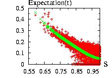
Fit of the expectation (green) for t=T/2 with a fourth order polynomial.
You can observe the dispersion of the option (red).
We have developped a class MonteCarloAmerican
to treat the American options. The declaration of the class can be found
in the file "MonteCarloAmerican.hpp". After created an instance with:
MonteCarloAmerican instance_MCA;
You could use different options: initial prices, correlations, interest rate,
…
The accessible functions (after a creation of an instance) are:
|
MonteCarloAmerican set_r(const double& r) MonteCarloAmerican set_S_ini(const vector<double>& s_ini) MonteCarloAmerican set_S_sigma(const vector<double>&s_sigma) MonteCarloEuropean set_Mu(const vector<double>&mu) MonteCarloAmerican set_Correlations(const vector<vector<double> >& correlations) MonteCarloAmerican set_PCA_Percent(const double& PCA_percent) MonteCarloAmerican set_n_Poly(const int& n_Poly) |
|
r is the constant interest rate |
|
MonteCarloAmerican set_Payoff(double payoff(const vector<double>& S,const vector<double>& Variables) ) MonteCarloAmerican set_Variables(const vector<double>& variables) MonteCarloAmerican set_function_Variables(void function_variables(vector<double>& S,vector<double>& Variables, const double& t) ) |
|
S={S0,S1,…} : stock price at time t |
| void initialize() |
|
Initialize the Monte Carlo defined with the set functions. Should always be used. |
| string information( ) |
|
Gives information about the Monte Carlo. |
|
void MonteCarlo(const double& t, const double& T, const double& Nt, const double& NMC) double Res_MC double Res_MC_error |
|
t is the present time (usually 0) |
To avoid overflow it could be better to divide the initial price and
the payoff by a factor and multiply the result after the MonteCarlo.
Example:
S0=110, E=100, payoff=max(S-E,0) ⇒ res=MonteCarlo
S0'=110/100=1.1, E'=100/100=1, payoff=max(S'-E',0) ⇒ res = 100*MonteCarlo
We have two assets S0 and S1 and
a payoff=max( max(S0(t),S1(t)) - E, 0 ).
The binomial method gives 13.90 [Boyle1989].
Example of program:
// Example MonteCarlo10.cpp
// Maximum of two assets

#include "LOPOR.hpp"
using namespace LOPOR;

double E=100.;       // strike
double r=0.05;       // interest rate
double D0=0.10;      // dividend
double S0=100.;      // initial price
double sigma=0.2;    // volatility
double T=3;          // expiry
double t0=0.;        // initial time
int    Nt=10;        // Nb of time interval between t0 and T
int    NMC=100000;    // number of MC


double payoff(const std::vector<double>& S, const std::vector<double>& Variables)
{
    return Max(Max(S[0],S[1])-E,0.);
}

int main( )
{
    try
    {

            // instance + initialization
        MonteCarloAmerican MCA;

            // r
        MCA.set_r(r);

            // S, sigma
        int NS=2;
        std::vector<double> S_ini=vec_create(NS,S0);
        std::vector<double> S_sigma=vec_create(NS,sigma);
        std::vector<double> Mu=vec_create(NS,r-D0);
         // correlation matrix Sigma':
        double rho1=0.0;
        double rho2=0.;
        std::vector<std::vector<double> > Correlations;
        Correlations=c2m(
                c2v(1.,rho1),
                c2v(rho1,1.)
                );

             // S, sigma, correlations
        MCA.set_S_ini(S_ini);
        MCA.set_S_sigma(S_sigma);
        MCA.set_Mu(Mu);
        MCA.set_Correlations(Correlations);

            // Polynomial fit order
        MCA.set_n_Poly(3);

            // payoff
        MCA.set_Payoff(payoff);

        MCA.initialize();  // you need to run it
        print(MCA.information()); //display information

        MCA.MonteCarlo(t0,T,Nt,NMC);

        // result with Monte Carlo
        print("Monte Carlo            =",MCA.Res_MC,"+/-",MCA.Res_MC_error);
        print("Binomial method        = 13.90");

    }
    catch (const Error& error) { error.information( ); }
    return 0;
}
And the output is:
MonteCarloAmerican initialization
S(t=0) :{100,100}
sigma  :{0.2,0.2}
mu     :{-0.05,-0.05}
PolynomialMulti order=3
Interest rate r      =0.05
Correlations:
1 0
0 1
PCA_Percent=1 which correspond to 2 dimensions
    eigenvalues: {1,1}
     normalized: {0.5,0.5}
              %: {0.5,1}

Monte Carlo            = 13.8787 +/- 0.0473272
Binomial method        = 13.90
We calculate the value of an American
Asian option for NS=4 stocks with correlations between them. We use
the principal component analysis to accelerate the simulation with
a precision of 97%
using the NormalMultiPCA class.
payoff=max( (Av0 + Av1 + … AvNS-1)/NS -E , 0)
with Avi = ∑t=0,TSi(t).
The program:
// Example MonteCarlo11.cpp
// American Asian option (arithmetic average) for 4 stocks
// at 97% for the PCA (Principal Component Analysis)

#include "LOPOR.hpp"
using namespace LOPOR;

double Norm=100;     // N=Normalization to avoid overflow
double E=100./Norm;  // strike
double r=0.10;       // interest rate
double D0=0.00;      // dividend
double S0=100./Norm; // initial price (for all stocks)
double sigma=0.2;    // volatility
double T=1.;         // expiry
double t0=0.;        // initial time
int    Nt=20;        // Nb of time interval between t0 and T
int    NMC=1000;    // number of MC


double payoff(const std::vector<double>& S, const std::vector<double>& Variables)
{
    return Max(E-Variables[0]/Variables[1],0.);
}

// Av = Average on time and on stocks
void function_Variables(std::vector<double>& S, std::vector<double>& Variables, const double& t)
{
    Variables[0] += vec_norm(S)/S.size();
    Variables[1] += 1;
}

int main( )
{
    try
    {

            // instance + initialization
        MonteCarloAmerican MCA;

            // S, sigma
        int NS=4;
        std::vector<double> S_ini=vec_create(NS,S0);
        std::vector<double> S_sigma=vec_create(NS,sigma);

         // correlation matrix Sigma':
        double rho1=0.95;
        double rho2=0.05;
        std::vector<std::vector<double> > Correlations;
        Correlations=c2m(
                c2v(1.,rho1,rho2,rho2),
                c2v(rho1,1.,rho2,rho2),
                c2v(rho2,rho2,1.,rho1),
                c2v(rho2,rho2,rho1,1.)
                );

             // S, sigma, correlations
        MCA.set_S_ini(S_ini);
        MCA.set_S_sigma(S_sigma);
        MCA.set_Correlations(Correlations);
        MCA.set_PCA_Percent(0.97);

            // Polynomial fit order
        MCA.set_n_Poly(3);

            // r, payoff
        MCA.set_r(r);
        MCA.set_Payoff(payoff);

            // 2 variables: the sum of the spin and the number of sum
        MCA.set_Variables(c2v(0.,0.));
        MCA.set_function_Variables(function_Variables);

        MCA.initialize();  // you need to run it
        print(MCA.information()); //display information


           // result with Monte Carlo
           // multiply by the normalization to get back the real price
        MCA.MonteCarlo(t0,T,Nt,NMC);
        print("Monte Carlo res=",Norm*MCA.Res_MC,"+/-",Norm*MCA.Res_MC_error);

    }
    catch (const Error& error) { error.information( ); }
    return 0;
}
And the output is:
MonteCarloAmerican initialization
S(t=0) :{1,1,1,1}
sigma  :{0.2,0.2,0.2,0.2}
mu     :{0.1,0.1,0.1,0.1}
Interest rate r      =0.1
PolynomialMulti order=3
Correlations:
1 0.95 0.05 0.05
0.95 1 0.05 0.05
0.05 0.05 1 0.95
0.05 0.05 0.95 1
PCA_Percent=0.97 which correspond to 2 dimensions
    eigenvalues: {2.05,1.85,0.05,0.05}
     normalized: {0.5125,0.4625,0.0125,0.0125}
              %: {0.5125,0.975,0.9875,1}

Monte Carlo res= 1.66197 +/- 0.0771742
This work was developped by [Barraquand1995].
The estimate is slightly high-biased.
The objective is to work backward in time, from T to t0,
to calculate the option using in a similar way as the binomial
model:
Vi(t) = e-r δt ∑i
pi→j(t) Vj(t+δt)
with δt a small interval of time, and the indices i and j
correspond to some states to define.
pi→j(t) is the
probability to be in the state i at time t and then in the state j
at time t+δt. We first calculate by Monte Carlo the probabilities
pi(t) and then we apply the condition:
Vi(t) = Max(Vi(t),payoffi(t))
For example imagine that we want to calculate an American put
with exercise price E=20 and S(t=0)=S0=10.
This procedure will become exact if the number of
interval of time Nt, the number of bins Ni
and the number of Monte Carlo NMC divided by Ni,
NMC/Ni,
are infinite. We present thereafter
an example of program.
What are the requirement of this procedure? The biggest problem is
a problem of memory to record bi,j(t), i.e. an array
of Nt*Ni*Ni.
However we can reduce considerably this
array remarking that the new spin S(t+δt) has a probability
near 0 to reach some state j, and therefore it is enough to record
the j around the actual state i. The new state j will be
more restricted if δt is small, i.e. Nt is large.
The requirement of memory is therefore only Nt*Ni*factor,
the factor could be 10 or something like that.
Now if we implement this algorithm we will observe that it is
not stable when Ni changes. Barraquand and Martineau
[Barraquand1995] introduced what
they called the Stratified State
Aggregation along the payoff. It consists to discretize the payoff space
and not the S space. With this stratification, results are very stable
for one variable:
The static function available is:
|
static vector<double>
Options::StateAgregationMonteCarlo(double S0,double E,double T,double t0,double r,double sigma,double NMC,double Nt)
|
|
Return a vector {value of MC, error} |
// Example MonteCarlo8.cpp
// American Put
// using the Statisfied State Aggregation

#include "LOPOR.hpp"
using namespace LOPOR;

double T=1, t0=0., r=0.05, sigma=0.20, D0=0., E=10., S0=9;

double payoff(const double& S) { return Max(E-S,0.); }
std::vector<double> monteCarlo( );

int main( )
{
    try
    {
        // Monte Carlo
        int NMC=100000;
        int Nt =10;
        double V=LOPOR::Options::StateAgregationMonteCarlo(S0,E,T,t0,r,sigma,NMC,Nt)[0];

        //Binomial method
        int    Nt_Binomial=1000;
        double BS_A=Options::Binomial(payoff,S0,Nt_Binomial,T,t0,r,sigma,D0,"American");

        // European option
        double BS_E=Options::European_Put(S0,E,T,t0,r,sigma,D0);

        print("S0=",S0,", by MC=",V,", Binomial=",BS_A,", European=",BS_E);

    }
    catch (const Error& error) { error.information( ); }
    return 0;
}
And the results are:
S0= 9 , by MC= 1.14941 , Binomial= 1.14937 , European= 1.02142
To estimate the error you should run several Monte Carlo, and estimate
the error from these results.
Flaws of the algorithm
The biggest problem using this algorithm is that it cannot give
an accurate result if we cannot include all information in the
stratification ("you cannot have your own cake and eat it").
Indeed if the correct behavior (hold or exercise the option)
depends not only of the payoff but also of the other parameters
you cannot expect that your stratification will work perfectly.
For example [Coyle1999].
In this article the authors proved that the SSAP cannot give a
correct results for a Put of the maximum or minimum of two
or three assets. You can then add a second dimension to your stratification
but you should know which one introduced, and, if you have to add
a third, fourth, … dimension the method will be impractical.
Raymar and Zwecher [Raymar1997 ]
have introduced a second dimension to treat the
call option on the maximum of several stocks.
This algorithms was developped by Broadie and Glasserman
[Broadie1997]. It is very similar to the Binomial or more
precisely to the b-nomial model where b is not restricted to
two. The idea is to simulate by Monte Carlo a tree with
b branches in a similar way of
the binomial model. At each time b random number
from the normal distribution are taken. Now we can construct a high-biased
and low-biased estimate calculating the option using (b-1) or b branches
at each time, respectively.
Biased low:
V(T)=payoff(S(T))
V(t)=max(payoff(S(t),discount/b ∑j=1b Vj(t+1)
Biased high:
V(T)=payoff(S(T))
V(t)=1/b ∑j=1b ηj
ηj = payoff(S(t)) if payoff(S(t)) > discount/(b-1)
∑i=1≠jb Vj
ηj = discount * Vj(t+1) otherwise
The flaws of this algorithms is that it is
exponentially time and memory consuming. Therefore it is restricted
to small dimensional problems. Moreover, the advantages compared
to the binomial
model are not striking: The binomial model is constructed in
a way that the two
branches model best the Normal distribution and therefore this
last model will give a better answer that the present algorithm. The only
advantage is that the errors can be calculated easily in this model,
however these are large. Therefore I do not advice to use these algorithms.
However there is no difficulties to implement them.
For a comparison of these
methods with other Monte Carlo see [Fu2001].
The idea of the algorithms using this method is to parameterize the boundary
condition where we exercise the option. For example for a simple
American put, the option will be exercised if the price of the option
S(t) < θ(t). When we discretize the time in K step we obtain
K unknown quantities. The objective is to maximize the option.
We can therefore derive a very simple algorithm:
To maximize the payoff you can use the Powel
function or the Annealing class.
The flaws of the methods are:
The biggest advantage of the methods is that the value of the option
is not so dependent of the value of the θ. The errors on
θ do not sum to produce a big error like in a backward time
algorithm.
You can get a high and low biased estimate
[Garcia2003].
The high biased estimate
is given by the maximum option calculated to get the "best" values
of the θ. A low biased estimate can be obtained using these
correct θ and redo a Monte Carlo to calculate the option. For large
number of Monte Carlo the biased will be very small.
For a comparison of these
methods with other Monte Carlo see [Fu2001].
We could improve the speed of the Monte Carlo defined a general rule
for the boundaries(t), for example a Bezier function with only
4 parameters (to be compared to Nt in the normal case). The point is
to have a rough idea of the form of the boundaries.
See [Cobb2004]
for more details.
[Ameur2002] use a related method to study
American Asian options.
An example of program to calculate a simple American put:
// Example MonteCarlo9.cpp
// American Put
// using the Parametric exercise boundary algorithm
// WITHOUT OPTIMIZATION

#include "LOPOR.hpp"
using namespace LOPOR;

double T=1, t0=0., r=0.05, sigma=0.20, D0=0., E=10., S0=9;
int    Nt=200;
std::vector<std::vector<double> > S;
bool   ini_MC=false;

double payoff(const double& S) { return Max(E-S,0.); }
std::vector<double> monteCarlo(const std::vector<double>& theta);

// UGLY
double FunctionMax(const std::vector<double>& theta)
{
    static double v=0.;
    for(int it=0; it< theta.size(); ++it)
        if(theta[it]>E) return -0.8*v;      // theta must be <= E for t<T
    for(int it=1; it< theta.size(); ++it)
        if(theta[it]<theta[it-1]) return -0.8*v;    // theta(t1) <= theta(t2) if t1 <t2

    // calcul MC et minus because we want the maximum
    v=monteCarlo(theta)[0];
    return -v;
}

int main( )
{
    try
    {
        print();
        print("S0=",S0);
        print();

        // number of temperatures
        Nt=20;

        // initial theta : Nt+1 value but the last one is fixed: theta(Nt+1)=E
        std::vector<double> theta(Nt);
        theta=vec_create3(0.7*E,0.99*E,Nt);

        double V;   // option

        // initial theta
        vec_print_1(vec_append(theta,E),"theta ini=");

        // maximum: find theta
        theta=MathFunctions::Minimize(FunctionMax,theta,1.e-10);
        vec_print_1(vec_append(theta,E),"theta fin=");

        // high bias
        V=monteCarlo(theta )[0];
        print();
        print("high bias by MC=",V);

        // low bias : redo the MC with new states
        ini_MC=false;
        V=monteCarlo(theta )[0];
        print("low bias  by MC=",V);

        //Binomial method
        int    Nt_Binomial=1000;
        double BS_A=Options::Binomial(payoff,S0,Nt_Binomial,T,t0,r,sigma,D0,"American",false);

        // European option
        double BS_E=Options::European_Put(S0,E,T,t0,r,sigma,D0);

        print();
        print("Binomial=",BS_A);
        print("European=",BS_E);
    }
    catch (const Error& error) { error.information( ); }
    return 0;
}

std::vector<double> monteCarlo(const std::vector<double>& theta1)
{
    int    NMC=10000;
    double dt=(T-t0)/c2d(Nt);
    double discount=exp(-r*dt);
    // theta(T) = E
    std::vector<double> theta=vec_append(theta1,E);

    int it, iMC;
    double Option=0.;

    if(S0<theta[0]) return c2v(payoff(S0));

    // first time create the stock price
    if(ini_MC==false)
    {
        S=matrix_create(NMC,Nt+1,S0);
        for(iMC=0; iMC< NMC; ++iMC)
        {
            for(it=1; it<= Nt; ++it)
            {
                S[iMC][it]=S[iMC][it-1]*exp((r-power(sigma)/2.)*dt
                  +sigma*sqrt(dt)*Normal::static_ran(););
            }
        }
        ini_MC=true;
    }

    for(iMC=0; iMC< NMC; ++iMC)
    {
        double V=0.;
        double Discount=1.;
        for(it=1; it<= Nt; ++it)
        {
            Discount *= discount;
            if(S[iMC][it]<theta[it])
                break;
        }

        Option += Discount*payoff(S[iMC][Min(it,Nt)]);
    }

    Option /= c2d(NMC);

    return c2v(Option);
}
And the output is:
S0= 9

theta ini= 7 7.145 7.29 7.435 7.58 7.725 7.87 8.015 8.16 8.305 8.45 8.595 8.74 8.885 9.03 9.175 9.32 9.465 9.61 9.755 9.9 10
theta fin= 6.76393 6.90893 7.78941 7.79176 8.07075 8.07607 8.20871 8.20986 8.22409 8.33742 8.36653 8.694 8.92897 8.94997 8.97504 9.05833 9.22434 9.34147 9.39085 9.63542 9.86024 10

high bias by MC= 1.15589
low bias  by MC= 1.14056

Binomial= 1.14923
European= 1.02142
IN CONSTRUCTION
I am currently developing the library including various models. For more
information refer to
[Brigo2001b,James2001,Rebonato2004a]
For one dimensional option, it is not really necessary to use the martingale
theory. However for higher dimension it is much more efficient, and for interest
rate derivatives options it is fundamental to use it. The reader should have
read the section Simple binomial model before
reading this section.
In this section we will not try to give a complete picture of the martingale, or the
Girsanov's theorem. We will try only to explain
the concepts using examples. No demonstration will be provided. The reader
interested in them should refer to [Joshi2003] for an
understandable (from my point of view) review or [Nielsen1999]
for a more formal approach.
The martingale is strongly connected to the
risk-neutral measures.
We have introduced it using the result of the
Black-Scholes equation. Indeed since the
risk of the stock μ does not appear in the equation but only r we can
replace r whenever μ appears. We will generalize this concept.
We first begin with one action S and one zero coupon bond B. The equations are:
dS = μ S dt + σ S dW = μ S dt + σ S ε dt½
dB = r B dt
with ε a random variable from a Normal(0,1) distribution.
We note that we can write:
S(t) = S(0) e(μ - σ2/2) t + σ ε t½
B(t) = B(0) er t
We can calculate:
d(S/B) = dS / B + S d(1/B) + dS d(1/B)
keeping only the order dt½ and dt we obtain:
d(1/B) = - r dt / B
d(S/B) = (μ - r) S/B dt + σ S/B ε t½
Now we define a martingale as a the quantity d(S/B) is driftless (the average is
constant). This force
μ = r
We note that B/B = 1 and therefore B is automatically a martingale.
The definition is therefore:
X is a martingale if, at least, it is driftless, i.e. d(X) = 0.dt + σ.dW
We can generalize the procedure if we are interested in f, a non tradable quantity, but fA and A are tradable. This is done in the section Particular martingales. More generally if B is tradable, and AB is tradable, then we have B/N and AB/N are martingale (i.e. driftless), N being the numeraire. From B/N we found the relation between the numeraire and B, and from AB/N between AB and N. Then we can calculate the drift of A as function of B parameters.
The change of numeraire is a change of variable.
In the previous section we took B as numeraire and considered B/B and S/B.
We now take S as numeraire and consider B/S and S/S. S/S=1 is a martingale.
What is the condition for B/S? Using this formula:
d(B/S) = dB/S + B.d(1/S) + dB.d(1/S)
d(B/S) = r B dt/S + B (-dS/S2 + dS2/S3) + neglect
d(B/S) = (r - μ + σ2) B dt/S - σ B/S ε t½
Now it is a martingale only if
μ = r + σ2
How can we reconcile this result with the one in the previous section (μ=r)?
The key point is that the estimation of the option will be similar.
We have define the condition on μ for the martingale following
the numeraire B, i.e. μ=r. We can now calculate the option V using:
V(t)/B(t) = Average(V(T)/B(T))
For a Vanilla Call we have
B(t) = B(0) ert
B(T) = B(0) erT
S(t) = S(0) e(r - σ2/2) t + σ ε t½
V(T) = max(S-E,0)
and we obtain:
V(t) = er(t-T)
(2 π)-½ ∫-∞+∞
dx.e-x2/2
max(S(t).er(T-t) - σ2(T-t)/2 + σ (T-t)½ x-K , 0)
Using the formula:
a x2 +b x +c = a (x + b/2a)2 −b2/4a + c
It is not difficult to find the
Black-Scholes result.
We now take the numeraire S, i.e. μ = r + σ2
S(t) = S(0) er t + σ ε t½
V(t)/S(t) = Average(V(T)/S(T))
V(t)/S(t) = Average(max(S(T)-K,0)/S(T))
V(t)/S(t) = Average(1-K/S(T)) when S(T) ≥ K
and we find a similar result.
This section was inspired from the chapter 7.8 from
Rebonato2004a .
We are interested to find the drift for a non tradable quantity f, but with
fA and A are tradable quantities. f could be a swap or a forward rate and
A a bond, for example. Our objective is to find the drift μf
in the measure associated to the numeraire N.
If fA and A are tradable, Z=fA/N=fX and X=A/N are martingales, i.e. driftless.
We have:
df = μf(f,t) dt + σf(f,t) dwf
= μf(f,t) dt + σf(f,t) εfdt½
dX = σX(X,t) dwX
= σX(X,t) εXdt½
dZ = σZ(Z,t) dwZ
= σZ(Z,t) εZdt½
But we can use Ito's Lemma to express dZ:
dZ = d(fX) = df X + f dX + df dX
dZ = (X μf(f,t) + σf(f,t) σX(X,t) εf εX ) dt + (X σf(f,t) εf + f σX(X,t) εX ) dt½
dZ = (X μf(f,t) + σf(f,t) σX(X,t) ρfX ) dt + (X σf(f,t) εf + f σX(X,t) εX ) dt½
Since we know that Z is a martingale, it has no drift term and we have:
X μf(f,t) + σf(f,t) σX(X,t) ρfX = 0
Now if we admit that f and X follow a lognormal distribution
we have f and X follow a geometric Brownian stochastic equation with:
μf(f,t) = f μf(t)
σf(f,t) = f σf(t)
μX(X,t) = X μX(t)
σX(X,t) = X σX(t)
and we obtain:
μf(t) = - σf σX ρfX
μf(t) = - σf σA ρfA + σf σN ρfN
We can find the Black-Scholes result
for Vanilla option
using the concept of martingale and
not the direct
partial differential approach using arbitrage of portfolio.
The two approaches are however equivalent as we will show it
thereafter.
The equivalent of the two approaches can also be seen
in the case of a Simple binomial model.
This section is equivalent to the one
for the simple binomial model.
Choice of numeraire: 1/B
dB = r B dt
d(1/B) = -dB/B2 + dB/B3 + … = -r dt/B
dS = μ S dt + σ S dt½ ε
d(S/B) = dS/B + S d(1/B) + dS d(1/B)
d(S/B) = μ S/B dt + σ S/B dt½ ε - S/B r dt + …
d(S/B) = (μ -r) S/B dt + σ S/B dt½ ε
But S/B is a martingale if
S(0)/B(0) = Average(S(t)/B(t))
or equivalently:
Average(d(S/B))=0.
Since Average(ε)=0 we must have
μ = r
we have :
dB = r B dt
dS = r S dt + σ S dt½ ε
Therefore:
B(t) = B(0) er t
S(t) = S(0) e(r-σ2/2) t + σ t½ ε
In the numeraire 1/B, V the option is a martingale:
V(0)/B(0) = Average(V(T)/B(T))
With
V(T) = (S(T) - E)+
V(T) = S(T) - E if S(T) ≥ E
But we have:
S(t) = S(0) e(r-σ2/2) t + σ t½ ε
Therefore the condition S(T) ≥ E is equivalent to:
(r-σ2/2) T + σ T½ ε ≥ log(E/S(0))
ε ≥ ( log(E/S(0)) - (r-σ2/2) T ) / (σ T½)
ε ≥ -d2
d2 = ( log(S(0)/E) + (r-σ2/2) T ) / (σ T½)
We can now calculate the option replacing the Average by the integration over
all possible final states, i.e. integration over the ε with the
associated probability e-ε2/2/(2π)½.
Using x=ε and B(T) = B(0) er T, we obtain:
V(0) = B(0)/(B(0)erT) ∫-d2∞
(S - E) e-x2/2 dx /(2π)½
V(0) = e-rT S(0) I1 + e-rT E I2
The calcul of the integrale I2 is extremely simple:
I2 = ∫-d2∞
e-x2/2 dx /(2π)½
I2 = ∫-∞d2
e-x2/2 dx /(2π)½
I2 = FNormal(d2)
The integral I1 is sligthly more complicated:
I1 = ∫-d2∞
e-x2/2 e(r-σ2/2) T + σ T½ x dx / (2π)½
I1 = ∫-∞d2
e-x2/2 e(r-σ2/2) T - σ T½ x dx / (2π)½
I1 = e(r-σ2/2) T
∫-∞d2
e-(x2 + 2 σ T½ x)/2 dx / (2π)½
I1 = e(r-σ2/2) T
∫-∞d2
e-(x+σ T½)2/2 + σ2T/2 dx / (2π)½
I1 = er T
∫-∞d2
e-(x+σ T½)2/2 dx / (2π)½
We have the change of variable y = x+σ T½
I1 = er T
∫-∞d2+σT½
e-y2/2 dy / (2π)½
I1 = er T FNormal(d1)
d1 = d2 + σ T½
d1 = ( log(S(0)/E) + (r-σ2/2) T ) / (σ T½) + σ T½
d1 = ( log(S(0)/E) + (r+σ2/2) T ) / (σ T½)
The result of the option at time 0 is therefore:
V(0) = e-rT S(0) I1 + e-rT E I2
V(0) = S(0) FNormal(d1)
- E e-rT FNormal(d2)
with:
d1 = ( log(S(0)/E) + (r+σ2/2) T ) / (σ T½)
d2 = ( log(S(0)/E) + (r-σ2/2) T ) / (σ T½)
Which is indeed the Black-Scholes result.
In this section we find an easier derivation of the
Black-Scholes result. The "difficult" part of
the last derivation was the calcul of I1. We will see that we
can avoid almost all calculations. The key point is to rewrite the
payoff of the option at time T as:
V(T) = (S(T) -E)+ = S(T) θ(S(T)-E) - E θ(S(T)-E)
where θ(x) is the Heaviside function which
return 0 if x ≤ 0 and 1 if x > 0. The option can therefore
be written as:
V = V1 - V2
To calculate V2 with a payoff V2(T)=E θ(S(T)-E)
we use the numeraire 1/B as previously. In this numeraire the rate μ of S
equal to r: μ=r and the stock price S can be written as:
S(t) = S(0) e(r-σ2/2) t + σ t½ ε
The condition S(T)-E > 0 can be written as
previously:
x > -d2
d2 = ( log(S(0)/E) + (r-σ2/2) T ) / (σ T½)
The martingale for V2 is:
V2(0)/B(0) = Average(V2(T)/B(T))
And the average for V2 under the form of an integrale can be calculated
as previously using B(T)=B(0)erT.
The result is:
V2 = E e-rT FNormal(d2)
To calculate V1 with a payoff S(T) θ(S(T)-E) we use
1/S as numeraire. In this numeraire we need to recalculate μ the rate of S
which will not be equal to r.
a. Calcul of μ. We have:
d(B/S) = dB/S + B d(1/S) + dB d(1/S)
and we have:
dS = μ S dt + σ S ε dt½
d(1/S) = -dS/S2 + dS2/S3 + …
d(1/S) = -(μ dt + σ ε dt½) dt S/S2
+ σ2 ε2 dt S2/S3
d(1/S) = (μ + σ2 ε2) dt/S - σ�ε dt½/S
Therefore:
d(B/S) = + r B dt/S + B ((μ + σ2 ε2) dt/S - σ ε dt½)/S + …
d(B/S) = (r + σ2 ε2 - μ) dt B/S
- σ ε dt½) B/S + …
B/S is a martingale if Average(d(B/S))=0, and using
Average(ε)=0 and Average(ε2)=1 we obtain that:
μ = r + σ2
b. Calcul of V1: V/S is a martingale therefore we have:
V1(0)/S(0) = Average(V1(T)/S(T))
V1(0) = S(0) Average(θ(S(T)-E))
The calcul of the average is similar to the one done previously for V2
but now we have μ = r + σ2 and not only r. S(T) is now:
S(t) = S(0) e(r + σ2 - σ2/2) t + σ t½ ε
S(t) = S(0) e(r + σ2/2) t + σ t½ ε
The condition S(T)-E > 0 can be written as
x > -d1
d1 = ( log(S(0)/E) + (r+σ2/2) T ) / (σ T½)
⇒ V1(0) = S(0) FNormal(d1)
The final result:
V(0) = V1(0) - V2(0)
V(0) = S(0) FNormal(d1)
- E e-rT FNormal(d2)
which is equivalent as the Black-Scholes result.
We have shown in the previous section that we can find
the Black-Scholes result
derived from the Partial differential equation (PDE)
using the martingale concept. We want to be more general and find the
Black-Scholes equation
from the martingale concept.
The idea is to use the numeraire 1/B and the fact
that the option is a martingale in this numeraire,
V(0)/B(0) = Average(V(T)/B(T))
or equivalently:
Average(d(V/B))=0
This last equation will give us the partial differential equation.
We begin to find the expression of d(V/B):
d(V/B) = dV/B + V d(1/B) + dV d(1/B)
We have:
d(1/B) = - r dt / B
and since V=V(S,t), using Ito's lemma:
dV = ∂V/∂t dt + ∂V/∂S dS
+ 1/2 ∂2V/∂S2 dS2 + …
But since (S/B) is a martingale, μ=r:
dS = μ S dt + σ S ε dt½
= r S dt + σ S ε dt½
Therefore:
dV = ∂V/∂t dt
+ ∂V/∂S (r S dt + σ S ε dt½)
+ 1/2 ∂2V/∂S2 σ2 S2 ε2 dt
dV = ( ∂V/∂t + r S ∂V/∂S + 1/2 ∂2V/∂S2 σ2 S2 ε2 ) dt
+ σ S ε dt½ ∂V/∂S
We obtain for V/B, keeping only the two first terms:
d(V/B) = ( ∂V/∂t + r S ∂V/∂S + 1/2 ∂2V/∂S2 σ2 S2 ε2 - r V ) dt/B
+ σ S/B ε dt½ ∂V/∂S
We apply now the condition that V/B is a martingale and therefore:
Average(d(V/B))=0.
Since Average(ε)=0 and Average(ε2)=1,
we must have:
∂V/∂t + r S ∂V/∂S + 1/2 σ2 S2 ∂2V/∂S2 - r V =0
Which is the Black-Scholes equation.
The Cameron-Martin's theorem concerns the change of variable
for stochastic variables when the path are distributed
as brownian motion with constant drift.
The Girsanov's theorem
treats the general case whith non constant drift.
Since I never understood this theorem untill I used it in one example,
I will introduce it using this way. This section used some results of
a course of Steve Lalley at the university of Chicago
[Lalley2001], lecture 8, and the chapter 8 of
the book of Mark Joshi [Joshi2003].
Before going to the example we will find the density of
W=t½ε whith ε distributed as
Normal(0,1). We have:
P(W < x) = P ( t½ε < x)
P(W < x) = P ( Norma(0,1) < x t½)
P(W < x) = (2 π)- ½
∫-∞xt½
e-s2/2 ds
P(W < x) = (2 π t)- ½
∫-∞x
e-s2/(2t) ds
Therefore the density of W, ρ(W) is:
ρ(W) = (2 π t)-½
e-s2/(2t)
We would like to calculate an European barrier option with a payoff at
time t=T:
payoff = Heaviside ( max(S(t))t=0,T > A )
We have, using the numeraire B, μS=r:
S(t) = S(0) e(r - σ2/2) t + σ ε t½
S(t) = S(0) e(r - σ2/2) t + σ W
The payoff can therefore rewritten as:
payoff = Heaviside ( max((r - σ2/2) t + σ W)t=0,T > log(A) )
payoff = Heaviside ( max((r - σ2/2) t /σ + W)t=0,T > log(A)/σ )
payoff = Heaviside ( max( θ t + W)t=0,T > α)
with
θ = (r - σ2/2)/σ
α = log(A)/σ
To calculate the option we have to average over all the expectations. Using
the fact that V/B is a martingale we arrive at:
V(t=0)/B(0) = Average(V(T)/B(T))
V(0) = e(-r T) Average(Heaviside ( max( θ t + W)t=0,T > α))
V(0) = e(-r T) Av
with
Av = Average(Heaviside ( max( θ t + W)t=0,T > α))
Av = (2 π T)- ½
∫-∞+∞
e-s2/(2T)
Heaviside ( max( θ t + s)t=0,T > α)
ds
Our problem is to calculate this average.
Unfortunately we cannot do it with this form of the Heaviside function. However
we know how to express (and so calculate the average)
the Heaviside function when θ=0:
Heaviside ( max(W)t=0,T > α)
Our objective is therefore to express our average as function of this
form. The obvious way is to do a change of variable:
W_ = θ t + W
s_ = θ t + s
the average becomes:
Av = (2 π T)- ½
∫-∞+∞
e-(s_ - θ t)2/(2T)
Heaviside ( max( s_)t=0,T > α)
ds_
Av = (2 π T)- ½
e-θ2 T / 2
∫-∞+∞
eθ s_
e-s_2/(2T)
Heaviside ( max( s_)t=0,T > α)
ds_
Av =
e-θ2 T / 2
Average(
eθ s
e-s2/(2T)
Heaviside ( max( s)t=0,T > α) )
And this average can be calculated using the reflexion principle.
Since our
objective is not to calculate the option I do not devlop the calculation
here and just quote the result:
Av =
e-θ2 T / 2
e+θ α
∫0∞
(eθx + e-θx)
e-(x+α2/2T
dx/(2 π T)½
and this integrale can be calculated using
FNormal.
We can now give a more formal definition of the Cameron-Martin's theorem.
W_ has a drift θ
W has no drift.
AverageW(event) = AverageW_(
e-θ2 t / 2 + θ W_ . event )
We can rewritte the term exponential term as dP/dP_ (P is the probability
associated to the measure W, and P_ to W_) called
sometimes the Radon-Nicodym derivative X:
X = e-θ2 T / 2 + θ W_
The drift is not constant. However we can redo almost a similar
demonstration as for the constant drif seen in the Cameron-Martin's theorem.
Simply the mathematics are a little bit more complicated
since, for example, you should write:
∫0t θ(s) dW(s)
and not
θ dW(t) as in the the constant drift. For a more detailled
description see [Lalley2001].
Simply compounded interest rate on a year basis:
Simply compounded interest rate on 1/n year basis:
Continuous compounded interest rate:
P(t,T) is the zero-coupon bond at date t with expiry T, i.e. discount value.
| rs(t,T) | (1/P(t,T) - 1) / (T-t) | simply-compounded spot rate |
| rτ(0,t) | ν (P(0,t)-1/νt - 1) | τ-period-compounded spot rate |
| rc(t,T) | -ln(P(t,T)) / (T-t) | continuously-compounded discrete spot rate |
| f(t,T1,T2) | (P(t,T1)/P(t,T2) - 1)/(T2 - T1) | simply-compounded forward rate |
| f(t,T,T+ΔT) | -(ln(P(t,T+ΔT) - ln(P(t,T)) / ΔT | continuously-compounded discrete forward rate |
| f(t,T) | -δln(P(t,T)/δT | instantaneous forward rate |
| r(t) | fc(t,t) | instantaneous spot rate |
|
static vector<double>
Options::Forward_rate
(vector<double> T, vector<double> P) |
|
Return the values (vector) of the forward rate = {f01,f12,…,fn-1,n} |
Example of program in Black_Flooret.cpp and in Black_Swaption.cpp.
The swap consists of
The part who pays the fixed rate is called the
payer's swap, the part
who pays the floating rate is called the
receiver's swap.
The set of floating payment is called the floating
leg, and the fixed payment is the fixed
leg.
The cash flow of the payer's swap at present value is:
Swap
= N ∑i=0N-1 τi fi P(Ti+1)
- N ∑i=0N-1 τi K P(Ti+1)
The fair interest rate X is when the present value is zero.
We obtain:
X = K(swap=0) = ∑i=0N-1τifi P(Ti+1
/ ∑j=0N-1 τj P(Tj+1)
X = K(swap=0) = ∑i=0N-1 wi fi
wi = τi P(Ti+1)/∑j=0N-1 τj P(Tj+1)
∑i=0N-1 wi = 1
We can also use the formula:
fij = ( P(Ti)/P(Tj) - 1 )/(Tj - Ti)
⇒ τi fi = τi fi,j=i+1 = ( P(Ti)/P(Ti+1) - 1 )=(P(Ti)-P(Ti+1))/P(Ti+1)
∑i=0N-1 P(Ti)-P(Ti+1)=P(T0) - P(TN)
to obtain:
X = (P(T0) - P(TN)) / B
B = ∑j=0N-1 τj P(Tj+1)
= annuity of the swap
Now we are at a latter time t but still before the
expiry date T0, the contract is no more 0.
Swap(t)
= N ∑i=0N-1 τi fi P(t,Ti+1)
- N ∑i=0N-1 τi K P(t,Ti+1)
We obtain:
Swapt = N (X - K)/B
B = ∑j=0N-1 τj P(Tj+1)
X = (P(T0) - P(TN)) / B
or X = ∑i=0N-1 wi fi
with wi = τi P(Ti+1)/∑j=0N-1 τj P(Tj+1)
and fi=fi,i+1
and fij = ( P(Ti)/P(Tj) - 1 )/(Tj - Ti)
We can express P(TN) as function of the swap rate X:
X = (P(T0) - P(TN)) / B
X = (P(T0) - P(TN)) / (∑j=0N-2 τj P(Tj+1)+tau;N-1 P(TN))
P(TN) =
(P(T0) - X ∑j=0N-2 τj P(Tj+1))
/ (1+tau;N-1X)
The static function available is:
|
static double
Options::Swap_rate
(vector<double> T, vector<double> P) static double Options::Swap_rate (vector<double> T, vector<double> P,double& B) |
|
Return X, the swap rate. |
Example of program in Black_Swaption.cpp.
A caplet is a call on rate K, i.e. a call on a FRA. The payoff
is therefore:
payoff= N max(f-K,0).(T2-T1).P(T2)
The option is exercised only if the fixed rate K < the floating rate f.
The forward rate f follows a lognormal distribution (in the Black model):
df = μ f dt + σ f dW = μ(t,t) f dt + σ f ε dt½
The problem to apply risk-neutral valuation is that f is not a traded asset.
I remind the reader that behind the concept is the hypothesis of
absence of arbitrage. But arbitrage is possible only if the asset is traded.
Therefore we need to find a traded asset with f. If the rate f is not traded,
the forward rate agreement FRA is a traded:
FRA = N (f-K) (T2-T1).P(T2)
But P(T2), a zero-coupon bond, is tradable we have that
f.P(T2) is tradable.
Now we take as numeraire P(T2) and
we know that in this numeraire a tradable asset/Numeraire
is a martingale:
TA/Numeraire = f.P(T2)/P(T2) = f
Since f is a martingale it is driftless, we have therefore:
df = σ f dW = σ f ε dt½
To estimate the value of the option C:
C(t=0)/P(0,T2) = Average( C(t=T1)/P(T1,T2) )
With P(t1,t2) is the zero-coupon bond at t1 with
expiry t2, or in other words, the present value at time t1
of a payment at time t2. We obtain:
C(f,t=0) = N P(0,T2) Average( max(f-K,0) ) (T2 - T1)
This is similar to a Black-Scholes call
with zero interest rate (r=0) and no dividend.
C(f,t,T1,T2) = N P(0,T2) (T2 - T1)
( f FNormal(d1)
− K
FNormal(d2))
with
d1 = [ log(f/K) + σ2 (T1−t)/2 ]/ [σ (T1−t)½]
d2 = [ log(f/K) − σ2)(T1−t)/2 ]/ [σ (T1−t)½]
The static function available is:
| static double Options::Black_Caplet (double K, double T1, double T2, double P1, double P2, double t, double σ, double Nominal=1) |
|
Return the value of the caplet |
Example of program in Black_Flooret.cpp.
A flooret is a put on rate K, i.e. a put on a FRA. The payoff
is therefore:
payoff= N max(K-f,0) (T2-T1).P(T2)
The option is exercised only if the fixed rate K > the floating rate f.
The formalism is therefore identical to the Black Caplet
replacing the call by a put.
Result is similar to a Black-Scholes put
with zero interest rate (r=0) and no dividend.
F(f,t,T1,T2) =
N P(0,T2) (T2 - T1)
(−f FNormal(−d1)
+ K
FNormal(−d2) )
with
d1 = [ log(f/K) + σ2 (T1−t)/2 ]/ [σ (T1−t)½]
d2 = [ log(f/K) − σ2)(T1−t)/2 ]/ [σ (T1−t)½]
The static function available is:
| static double Options::Black_Flooret (double K, double T1, double T2, double P1, double P2, double t, double σ, double Nominal=1) |
|
Return the value of the flooret |
Example of program:
// Example Black_Flooret.cpp

#include "LOPOR.hpp"

using namespace LOPOR;

int main( )
{
    try
    {
        double K=0.045;
        double T1=0.75;
        double T2=1;
        double P1=0.9632;
        double P2=0.9512;
        double t=0;
        double sigma=0.1;
        double Nominal=100;

        std::vector<double> T, P, Forward_rate;
        T=c2v(T1,T2);
        P=c2v(P1,P2);
        Forward_rate=Options::Forward_rate(T,P);
        print("forward rate=",Forward_rate[0]);

        double Black_Caplet=Options::Black_Caplet(K,T1,T2,P1,P2,t,sigma,Nominal);
        double Black_Flooret=Options::Black_Flooret(K,T1,T2,P1,P2,t,sigma,Nominal);

        print("Caplet with Black formula=",Black_Caplet);
        print("Flooret with Black formula=",Black_Flooret);

    }
    catch (const Error& error) { error.information( ); }
    return 0;
}
The output is:
forward rate= 0.0504626
Caplet with Black formula= 0.134152
Flooret with Black formula= 0.00425172
This section is very similar to the two previous ones. A swap can be written as:
Swap = N (X - K)/B
B = ∑j=0N-1 τj P(Tj+1)
K is the fixed interest
X is the "swap rate", i.e. a sum of different rates.
If we admit that the forward rate is lognormal, X cannot be lognormal, however
the difference will not be so strong. Therefore we admit that X follows a lognormal
distribution:
dX = μ X dt + σ X dW = μ(t,t) X dt + σ X ε dt½
Tradable asset.
We observe that X could be written as
X = (P(T0) - P(TN)) / B
B = ∑j=0N-1 τj P(Tj+1)
= annuity of the swap
Therefore X is constructed from zero-coupon bonds which are tradable, and so X is.
Numeraire. The best choice is to choose B as numeraire.
X becomes, in this numeraire, a martingale and a driftless quantity:
dX = σ X dW = σ X ε dt½
To estimate the value of the Swaption:
Swaption(t=0)/B(t=0) = Average( Swaption(t=T)/B(t=T) )
⇒ Swaption(t=0) = N B(t=0) Average(max(X-K,0)) for the payer's swap
This is similar to a Black-Scholes call
with zero interest rate (r=0) and no dividend.
Swaption(t,Ti,P(Ti)) = N B(t=0)
( X FNormal(d1)
− K
FNormal(d2))
with
d1 = [ log(X/K) + σ2 (T0−t)/2 ]/ [σ (T0−t)½]
d2 = [ log(X/K) − σ2)(T0−t)/2 ]/ [σ (T0−t)½]
The static function available is:
| static double Options::Black_Swaption (double K, vector<double> T, vector<double> P, double t, double σ, double Nominal=1) |
|
Return the value of the caplet |
Example of program:
// Example Black_Swaption.cpp

#include "LOPOR.hpp"

using namespace LOPOR;

int main( )
{
    try
    {
        std::vector<double> T, P, Forward_rate;
        T=c2v<double>(1,1.5,2.,2.5,3.,3.5,4.);
        P=c2v<double>(0.94999,0.92397,0.89803,0.87245,0.847375,0.82289,0.79904);
        double K=0.06;
        double t=0;
        double sigma=0.2;
        double Nominal=100;

        Forward_rate=Options::Forward_rate(T,P);
        vec_print(T,P,Forward_rate," T=     P=       Forward_rate f=");

        double Swap_rate=Options::Swap_rate(T,P);
        print("\nSwap rate=X=",Swap_rate);

        double Black_Swaption=Options::Black_Swaption(K,T,P,t,sigma,Nominal);
        print("\nSwaption with Black formula=",Black_Swaption);

    }
    catch (const Error& error) { error.information( ); }
    return 0;
}
The output is:
#   i=        T=     P=       Forward_rate f=
     0          1    0.94999  0.0563222
     1        1.5    0.92397  0.0577709
     2          2    0.89803  0.0586395
     3        2.5    0.87245  0.0591828
     4          3   0.847375  0.0595098
     5        3.5    0.82289  0.0596966
     6          4    0.79904

Swap rate=X= 0.0584652

Swaption with Black formula= 1.03023
A bond is a contract that yields
We admit that the interest rate r follows
a stochastic differential equation:
dr = u(r,t) dt + w(r,t) ε dt½
This equation is very similar to
the one for the asset S.
We can apply Ito's lemma
to the bond V(r,t):
with x=t, y=r, a=u; and b=w:
dV(r,t) = ∂V/∂r w ε dt½
+ (∂V/∂t + ∂V/∂r u + ½ w2 ∂2V/∂r2) dt + K dt + O(dt3/2)
K is the "coupon" (dividend) which van be continue or discrete (sum of δ).
Now we want to construct a portfolio to hedge our risk.
Hedging bonds is more difficult than assets because there is no
underlying asset with which to hedge. However we can overcome the problem
constructing a portfolio of several bonds at different maturity. Consider
the case of two bonds V1 and V2.
We holds V1 long, and Δ V2 short.
The portfolio Π is:
Π = V1 - Δ V2
Choosing Δ=∂V1/∂r/∂V2/∂r
, we can eliminate the random component ε and the
portfolio is wholly deterministic:
dΠ =
( ½ w2 ∂2V1/∂r2
+ ∂V1/∂t + K1
- Δ (½ w2 ∂2V2/∂r2
+ ∂V2/∂t + K2)
) dt
Now we consider that the market are efficient and no arbitrage is possible, i.e.
that the risk free profit of invest money Π, rΠdt, should be equal to dΠ.
Using the definition of Π = V1 -Δ V2, we arrive to:
( ∂V1/∂t +
½ w2 ∂2V1/∂r2
− r V1 + K1) / ∂V1/∂r =
( ∂V1/∂t +
½ w2 ∂2V2/∂r2
− r V2 + K2) / ∂V2/∂r
But V1(r,t,T1) depends of the maturity date T1,
and V2 of T2 therefore we can conclude that:
(∂V1/∂t +
½ w2 ∂2V1/∂r2
− r V1 + K1) / ∂V1/∂r = a(r,t)
and a similar equation holds for V2. Dropping the subscript
and rewriting
a(r,t) = w λ - u (all functions depend of r and t)
we obtain the equation:
∂V/∂t +
½ w2 ∂2V/∂r2
+ (u − λ w) ∂V/∂r − r V + K = 0
The problem is therefore similar to the options but we have first to found
the correct form of the functions u(r,t), w(r,t) and λ(r,t).
We can also introduce the yield Y(t,T)
curve which is a measure of future value
of interest rate as function of T, t, and the spot rate r:
Y(r,t,T) = - log(V(r,t,T)/V(r,T,T)) / (T-t)
In this section we are interested to find a
solution of the form:
V(r,t,T) = Z eA(t,T) -r B(t,T)
with A(T,T)=B(T,T)=0.
Introducing this equation in the
equation for bonds we obtain:
∂A/∂t - r ∂B/∂t + ½ w2 B2
- (u - λ w) B - r = 0
A and B depend of t and T, and u and w of r and t. Differentiating two
times by r this equation becomes:
½ B2 ∂2w2/∂2r
- B ∂2(u - λ w)∂2r = 0
or
½ B ∂2w2/∂2r
- ∂2(u - λ w)∂2r = 0
Since B is a function of T but not u, λ or w we, must have:
∂2w2/∂2r = 0
∂2(u - λ w)∂2r = 0
the form of w is from the first equation:
w(r,t) = ( α(t) r - β(t) )½
and from the second we can find the form of:
u - λ w = -γ(t) r + η(t)
The minus sign in front of β(t) and γ(t) are conventional.
We obtain therefore:
w(r,t) = ( α(t) r - β(t) )½
u(r,t) = -γ(t) r + η(t) + λ ( α(t) r - β(t) )½
Introducing this formula in the equation:
∂A/∂t - r ∂B/∂t + ½ w2 B2
- (u - λ w) B - r = 0
we obtain:
∂A/∂t - r ∂B/∂t + ½ (α(t) r - β(t)) B2
- (-γ(t) r + η(t)) B - r = 0
r ( - ∂B/∂t + ½ α(t) B2
+ γ(t) B - 1 )
+ ∂A/∂t - ½β(t) B2 - η(t) B = 0
Since A(t,T) and B(t,T) does not depend of r we obtain two equations:
∂A/∂t = ½β(t) B2 + η(t) B
∂B/∂t = ½ α(t) B2 + γ(t) B - 1
For this model the yield is:
Y(r,t,T) = - log(V(r,t,T)/V(r,T,T)) / (T-t)
Y(r,t,T) = - log(Z eA(t,T) -r B(t,T)/Z) / (T-t)
Y(r,t,T) = (- A(t,T) +r B(t,T)) / (T-t)
If α, β, γ, η are constant we can integrate the
equations and obtain:
B(t,T) = 2 f /
[
(γ + ψ1) f + 2 ψ1
]
f = eψ1 (T - t) - 1
ψ1 = (γ2 + 2 α)½
α A / 2 = a ψ2 log(a - B)
+ (ψ2 - ½ β) b log(1 + B/b)
+ ½ B β - a ψ2 log(a)
a = (-γ + ψ1)/α
b = (+γ + ψ1)/α
ψ2 = (η + a β/2)/(a + b)
With all parameters α, β, γ and η(t)
we can calculate A and B,
exactly for B(t,T), and numerically for A(t,T). And V(r,t,T) is
estimated using:
V(r,t,T) = Z eA(t,T) -r B(t,T)
The flaw of this model is that the parameters should be constant
which is surely not the case.
We define a bond option VB similarly as we define
the equity option as previously defined.
First we must calculate the value of the bond
solving the equation:
∂Bond/∂t +
½ w2 ∂2Bond/∂r2
+ (u − λ w) ∂Bond/∂r − r Bond = 0
With the condition B(r,T,T)=Z.
The bond option
depends of r and t: VB(r,t,T) and therefore follow the same equation
as the bond
∂VB/∂t +
½ w2 ∂2VB/∂r2
+ (u − λ w) ∂VB/∂r − r VB = 0
but with the final condition VB(r,T,T) = payoff.
u(r,t) and w(r,t) must be estimated using previous data and previsions.
A convertible bond V is an ordinary bond which can be exchanged for
a n specified asset S, usually at any time. This imply that :
V ≥ n S
if the number n << number of asset S in the market.
If the rate is constant the convertible bond is a function of the price
of the asset S, the time t, and the maturity date T, V(S,t,T).
We can construct a portfolio Π of one bond and −Δ asset S:
Π = V - Δ S
dΠ = dV - Δ dS - Δ D dt + K dt
where D is the continuous dividend of the asset S and K is the "coupon",
i.e. continuous dividend of the bond. Be careful that we have
D= D0 S with the notation of the section
Black-Scholes model with dividend.
Using Ito's lemma we obtain:
dΠ = ∂V/∂S dS - Δ dS
+ (∂V/∂t
+ ½ σ2 S2 ∂2V/∂S2 + K - Δ D S ) dt
choosing Δ = ∂V/∂S we eliminate the risk of the portfolio. This
riskless portfolio return cannot be larger than a bank deposit, rΠ=r(V - Δ S), from arbitrage
considerations, and we get:
∂V/∂t + ½ σ2 S2 ∂2V/∂S2 + (r S - D) ∂V/∂S - r V + K ≤ 0
The conditions are:
V(S,T,T) = Z (the principal)
V ≥ n S (from arbitrage)
V(S → ∞, t, T) ∼ n S
V(S=0, t, T) = Z e-r (T - t)
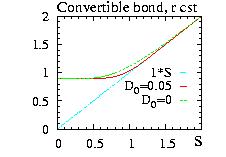
Z=1, n=1, σ=0.4, r=0.1, T=1 year, K=0
Example of program used to plot the figure:
// Example SOR_convertible_bond1.cpp
// r is constant, dividend D=D_0 S
// at one year of maturity

#include "LOPOR.hpp"
using namespace LOPOR;

double D_0=0.05, K=0, Z=1, sigma=0.4, r=0.1, T=1;
int n=1;   // convertible bond -> n S

// payoff for a Put
double payoff(const double& S)
{
    return Max(c2d(n)*S, Z);
}

// condition for an American put: V > payoff
double condition(const double& S, const double& utemp)
{
    return Max(utemp,c2d(n)*S);
}

int main( )
{
    try
    {

        std::vector<double> S=vec_create3(0.,3.,60);

        // dV/dt = a(x,t) d^2V/dx^2 + b(x,t) dV/dx + c(x,t) V + d(x,t)
        // coeff={a,b,c,d}
        // a ={a(x0),a(x1),…}, b={…}, …
        std::vector<std::vector<double> >
            coeff(matrix_create<double>(4,S.size(),0.));
        for(int i=0; i<S.size(); ++i)
        {
            coeff[0][i]=power(sigma*S[i])/2.;  // sign: Option t -> -t
            coeff[1][i]=r*S[i]-D_0*S[i];
            coeff[2][i]=-r;
            coeff[3][i]=K;
        }

        // V(S,t=T)
        std::vector<double> V(S);
        for(int i=0; i<S.size(); ++i)
            V[i]=payoff(S[i]);

        double dt=T/10.;
        int loops;

        for(double t=T; t>= -ERROR; t-=dt)
        {
            V[0]=payoff(S[0])*exp(-r*(T-t));  // boundaries S=0
            V[S.size()-1]=payoff(S[S.size()-1]);  // boundaries S=oo
            loops=PartialDiffEqs::SOR(S,dt,V,coeff,condition);
            print("t="+c2s(t)+":  number of loops=  "+c2s(loops));
        }

        print("Results wrote in file \"SOR_Bond1.res\": (i,S,Option)");
        vec_print("SOR_Bond1.res",S,V);
    }
    catch (const Error& error) { error.information( ); }
    return 0;
}
And the output is:
t=1:  number of loops=  17
t=0.9:  number of loops=  16
t=0.8:  number of loops=  16
t=0.7:  number of loops=  17
t=0.6:  number of loops=  17
t=0.5:  number of loops=  18
t=0.4:  number of loops=  18
t=0.3:  number of loops=  18
t=0.2:  number of loops=  18
t=0.1:  number of loops=  18
t=1.38778e-16:  number of loops=  18
Results wrote in file "SOR_Bond1.res": (i,S,Option)
∂V/∂t +
½ ( w2 ∂2V/∂r2
+ ½ S2 σ2 ∂2V/∂S2
+ 2 σ w ρ ∂2V/∂S∂r
)
+ (r S - D) ∂V/∂S
+ (u − λ w) ∂V/∂r − r V + K = 0
with D the dividend of S, and K the coupon of the bond V.
An interest rate swap is a contract which provides a variable interest rate r
of an amount Z while at the same time the buyer must give to the holder
a fixed interest rate r'. During the time dt the buyer will receive
the amount Z(r−r')dt.
Since the Swap(r,t,T) is a function of r it satisfy Ito's lemma and we can redo
the procedure we have done in the previous section.
However it is faster to remark that the amount received by the buyer,
Z(r−r')dt, can be seen as a "coupon" K dt of the bond and therefore the
swap satisfy:
∂Swap/∂t +
½ w2 ∂2Swap/∂r2
+ (u − λ w) ∂Swap/∂r − r Swap + Z (r - r') = 0
With the condition Swap(r,T,T) = 0 : all the principal Z must have been
paid at t=T.
A swaption is an option on a swap. Similarly to the option on bond we
observe that the swaption is a function of r and t and therefore obey
the same equation (but without the "dividend"):
∂Swaption/∂t +
½ w2 ∂2Swaption/∂r2
+ (u − λ w) ∂Swaption/∂r − r Swaption = 0
but with the final condition Swaption(r,T,T) = payoff.
A cap (floor) is a loan at the floating interest rate but
with a maximum (minimum) rate r'.
During the time dt the buyer will receive
the amount Z minimum(r,r')dt for a cap and Z maximum(r,r')dt for a floor.
Since the Cap(r,t,T) is a function of r it satisfy Ito's lemma and we can redo
the procedure we have done in the previous section.
However it is faster to remark that the amount received by the buyer,
Z minimum(r,r')dt, can be seen as a "coupon" K dt of the bond and therefore the
swap satisfy:
∂Cap/∂t +
½ w2 ∂2Cap/∂r2
+ (u − λ w) ∂Cap/∂r − r Cap + Z minimum(r,r')dt = 0
With the condition Cap(r,T,T) = 1 : all the principal Z must have been
received at t=T.
A caption is an option on a Cap. Similarly to the option on bond we
observe that the caption is a function of r and t and therefore obey
the same equation (but without the "dividend"):
∂Caption/∂t +
½ w2 ∂2Caption/∂r2
+ (u − λ w) ∂Caption/∂r − r Caption = 0
but with the final condition Caption(r,T,T) = payoff.
[Ameur2002]
H. Ben Ameur, M. Breton, and P. L'Ecuyer,
A Dynamic Programming Procedure for Pricing American-Style Asian Options
,
Management Science, 48 (2002) 625.
[Babbs2000]
S. Babbs,
Journal of Economic Dynamics & Control, 24 (2000) 1499
[Barraquand1995]
J. Barraquand and D. Martineau,
Numerical valuation of high dimensional
multivariate American securities,
Journal of Financial and Quantitative Analysis, 30 (1995) 383.
[Baxter1996]
M. Baxter, and A. Rennie,
Financial Calculus, an introduction to derivative pricing,
Cambridge university press, 1995
[Blitz++]
Object- Oriented Scientific Computing,
http://www.oonumerics.org/blitz/
[Boyle1977]
P. Boyle,
Journal of Financial Economics, 4 (1977) 323
[Boyle1989]
P. Boyle, J. Evnine, and S. Gibbs,
Numerical evaluation of multivariate contingent claims,
Review of Financial Studies, 2 (1989) 241
[Boyle1997]
P. Boyle, M. Broadie, and P. Glasserman,
Journal of Economic Dynamics and Control, 21 (1997) 1267
[Broadie1996]
M. Broadie and P. Glasserman,
Estimating security price derivatives by simulation,
Management Science, 42 (1996) 269.
[Broadie1997]
M. Broadie and P. Glasserman,
Pricing American-style securities using simulation,
Journal of Economic Dynamics and control, 21 (1997) 1323.
[Brigo2001a]
D. Brigo and F. Mercurio,
Displaced and mixture diffusion for analytically-tractable smile model,
Mathematical finance, Bachelier Congress 2000, Geman, H., Madan, D.B., Pliska, S.R., Vorst, A.C.F., eds. Springer Finance, Springer, Heidelberg..
[Brigo2001b]
D. Brigo and F. Mercurio,
Interest Rate Models: Theory and Practice,
Springer Finance, Heidelberg, 2001.
[Broyden1965]
C.G. Broyden,
Mathematics of Computation, 19 (1965) 577
[Cairo1997]
M.C. Cairo, and B.L. Nelson,
Modeling and generating random vectors with arbitrary marginal distributions and correlation matrix
Technical Report, Department of Industrial and Management Sciences, Northwestern University, Evanston, IL, 1997.
[Cavalli-Sforza1996]
L.L. Cavalli-Sforza, P. Menozzi, A. Piazza,
The History and Geography of Human Genes : (Abridged paperback edition) ,
Princeton University Press, 1996.
[Chancellor2000]
E. Chancellor,
Devil take the hindmost,
A plum book, penguin, 2000.
[Chen2001]
H. Chen,
Initialization for NORTA: generation of random vectors with specified marginals and correlations,
Journal on computing, 13 (2001) 312.
[Clewlow1998]
L. Clewlow and C. Strickland,
Implementing derivatives models,
ed. Wiley, 1998.
[Cobb2004]
B.R. Cobb and J.M. Charnes,
Approximating free exercise boundaries for American-style options
using simulation and optimization,
Proceedings of the 2004 Winter Simulation Conference,
Eds. R.G. Ingalls, M.D. Rosseti, J.S. Smith, and B.A. Peters.
[Cox1976]
J. Cox and S. Ross,
The valuation of options for alternative stochastic processes,
Journal of Financial Economics, 3 (1976) 145.
[Cox1985]
J. Cox and M. Rubinstein,
Option markets,
ed. Prentice Hall, 1985.
[Coyle1999]
L.N. Coyle and J.J. Yang,
Analysis of the SSAP Method for the Numerical Valuation of High-Dimensional Multivariate American Securities,
Algorithmica, 25 (1999) 75.
[Cruz2002]
M. G. Cruz,
Modeling, measuring and hedging operational risk,
ed. Wiley, 2002.
[Davison1997]
A.C. Davison, and D.V. Hinkley,
Bootstrap Methods and their Applications,
ed. Campbrige University Press, 1997.
[Derman1994]
E. Derman and I. Kani,
Riding on a smile,
Risk, 7 (1994) 32.
[Derman1995a]
E. Derman, D. Ergener, and I. Kani,
Static options replication,
Journal of derivatives, Summer (1995) 78.
[Dupire1994]
B. Dupire,
Pricing with a smile,
Risk, 7 (1994) 18.
[Efron1993]
B. Efron, and R.J. Tibshirani,
An Introduction to the Bootstrap,
ed. Chapman&Hall, 1993.
[Evans2000]
E. Evans, N. Hastings, and B. Peacock,
Statistical Distributions,
ed. Wiley, Third edition, 2000.
[Fu2001]
M. Fu, S.B.Laprise, D.B. Madan, Y. Su, and R. Wu,
Pricing American Options: A Comparison of Monte Carlo Simulation Approaches,
Journal of Computational Finance, 4 (2001) 39.
[Garcia2003]
D. Garcia,
Convergence and Biases of Monte Carlo estimates of American option prices using a parametric exercise rule,
Journal of Economic Dynamics and Control, 27 (2003) 1855.
[Gelman2000]
A. Gelman, J.B. Calin, H.S. Stern, and D.B. Rubin,
Bayesian Data Analysis,
ed. Chapman&Hall, 2000.
[Ghosh2002]
S.Ghosh and S.G. Henderson,
Properties of the NORTA method in higher dimensions,
Proceedings of the 2002 Winter Simulation Conference. E. Yucesan, C.-H. Chen, J. L. Snowdon, and J. M. Charnes, eds. IEE, 2002
[Glasserman1999]
P. Glasserman, P. Heiselberger, and P. Shahabuddin,
Mathematical Finance, 9 (1999) 117
[Glasserman2004]
P. Glasserman,
Monte Carlo methods in financial engineering,
Springler, 2004
[GnuLibrary]
A free/open-source C and C++ library numerical library,
http://www.gnu.org/software/gsl/
[Hornick1989]
K. Hornick, M, Stinchcombe and H. White,
Multilayer feedforward networks are universal approximators,
Neural Networks 2(1989) 359.
[Hull1997]
J. C. Hull,
Options, Futures, and Other Derivatives,
ed. Prentice-Hall, Third Ed., 1997.
[Jackel2002]
P. Jackel.
Monte Carlo method in finance,
Wiley, 2002.
[James2001]
J. James and N. Webber,
Interest rate modeling,
Wiley, 2001.
[Johnson1994a]
N. Johnson, S. Kotz, N. Balakrishnan,
Continuous Univariate Distributions,
ed. Wiley, Second edition, 1994.
[Johnson1994b]
N. Johnson, S. Kotz, N. Balakrishnan,
Discrete Univariate Distributions,
ed. Wiley, Second edition, 1994.
[Johnson1994c]
N. Johnson, S. Kotz, N. Balakrishnan,
Continuous Multivariate Distributions,
ed. Wiley, Second edition, 1994.
[Joshi2003]
M. Joshi,
The Concepts and Practice of Mathematical Finance,
Cambridge University Press.
[Joshi2004]
M. Joshi,
Design Patterns and Derivatives Pricing,
Cambridge University Press.
[Kindleberger2000]
C.P. Kindleberger,
Manias, panics, and crashes ,
Wiley, 4th edition, 2000.
[Lalley2001]
S. Lalley,
Statistics and Mathematical Finance,
unpublished, accessible at
http://www.stat.uchicago.edu/~lalley/Courses/390/.
[Kleinert]
H. Kleinert,
Path Integrals in Quantum Mechanics, Statistics,
Polymer Physics, and Financial Markets,
Wold Scientific, 3rd edition, 2004.
[Lepage]
G.P. Lepage,
Journal of Computational Physics, 27 (1978) 192
[Levy1997]
E. Levy,
Exotic options: the state of the art,
Ed. L. Clewlow and C. Strickland,
International Thomson Publishing, London, 1997.
[Loison2000]
D. Loison, and P. Simon,
Phys. Rev. B 61 (2000) 6114, appendix
[Loison2004]
D. Loison, C. Qin, K.D. Schotte, X.F. Jin,
Euro. Phys. J. B 41 (2004) 395,
accessible from
http://www.physik.fu-berlin.de/~loison/fast_algorithms/index.html.
[Loison2004b]
D. Loison,
http://www.physik.fu-berlin.de/~loison/fast_algorithms/index.html.
[London2005]
J. London,
Modeling derivatives in C++,
Wiley, 2005.
[Longstaff2001]
F.A. Longstaff and E.S. Schwartz,
Valuing American options by simulation:
a simple least-squares approach ,
The Review of Financial Studies, 14(2001) 113.
[Marshall2001]
C. Marshall,
Measuring and managing operational risk in financial institutions,
Wiley, 2001.
[Merton1976]
R.C. Merton,
Option pricing when underlying stock returns are discontinuous,
Journal of Financial Economics, 3(1976) 125.
[Newmat]
C++ Matrix library: http://www.robertnz.net/
[Newton1997]
N.J. Newton,
Numerical methods in Finance,
editors L.C.G. Rogers, and D. Talay,
Cambridge University Press, 1997.
[Nielsen1999]
L.T. Nielsen,
Pricing and hedging of derivative securities,
Oxford University press, 1999.
[Numerical Recipes]
W.H. Press, S.A. Teukolsky, W.T. Vetterling, and B.P. Flannery,
Numerical Recipes in C++,
Cambridge University Press, second ed., 2002.
http://www.library.cornell.edu/nr/cbookcpdf.html
A must for numerical calculations, even if programs are simply
a translation of FORTRAN.
[Peterson1979]
R. Kronmal and A. Peterson,
American Statistician, 33(1979) 214.
[Pizzi2002]
C. Pizzi, P. Pellizzari,
Monte Carlo Pricing of American Options Using Nonparametric Regression,
Rendiconti per gli Studi Economici Quantitativi, (2002) 75.
http://econwpa.wustl.edu/eprints/fin/papers/0207/0207007.abs
[QuantLib]
A free/open-source C++ library for quantitative finance,
http://www.quantlib.org/
[Raymar1997]
S. Raymar, M. Zwecher,
A Monte Carlo valuation of American call options
on the maximum of several stocks,
Journal of Derivatives 5(1997) 7.
[Rebonato2004a]
R. Rebonato,
Interest-rate option models,
ed. Wiley, Second edition, 2004.
[Rebonato2004b]
R. Rebonato,
Volatility and correlation,
ed. Wiley, Second edition, 2004.
[Sautter1996]
C. Sautter,
La Puissance Financiere du Japon,
Economica, 1996.
[Schoenmakers1997]
J.G. Schoenmakers, and A.W. Heemink,
Journal of Computational Finance, 1 (1979) 47.
[Silvia1996]
D.S. Silvia,
Data Analysis: a Bayesian Tutorial,
ed. Oxford University Press, 1996.
[Smith1965]
G.D. Smith,
Numerical Solution of Partial Differential Equations,
ed. Oxford University Press, 1965.
Old but a perfect introduction to the finite differences.
[Vapnik1999]
V.N. Vapnik,
The nature of statistical learning theory (statistics for engineering and information science),
Springler Verlag, 1999, 2nd ed.
[Sornette2004]
D. Sornette,
Why Stock Markets Crash : Critical Events in Complex Financial Systems,
ed. Princeton University Press, 2004.
[Vose2003]
D. Vose,
Risk analysis, a Quantitative Guide,
ed. Wiley, second edition, 2003.
[Wilmott2000]
P. Wilmott, J. Dewynne, and S. Howison,
Option pricing, mathematical models and computation,
ed. Oxford Financial Press, 2000.
Use the "Find" of your browser! Usually <Ctr F>
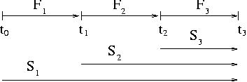